University of Warwick institutional repository: http://go.warwick.ac.uk/wrap
This paper is made available online in accordance with
publisher policies. Please scroll down to view the document
itself. Please refer to the repository record for this item and our
policy information available from the repository home page for
further information.
To see the final version of this paper please visit the publisher’s website.
Access to the published version may require a subscription.
Author(s): Adam M. Johansen, Arnaud Doucet and Manuel Davy
Article Title: Particle methods for maximum likelihood estimation in
latent variable models
Year of publication: 2007
Link to published article:
http://dx.doi.org/10.1007/s11222-007-9037-8
ESTIMATION IN LATENT VARIABLE MODELS
ADAM M. JOHANSEN, ARNAUD DOUCET AND MANUEL DAVY
Abstract. Standard methods for maximum likelihood parameter estimation in latent variable models rely on the Expectation-Maximization algorithm and its Monte Carlo variants. Our approach is different and motivated by similar considerations to simulated annealing; that is we build a sequence of artificial distributions whose support concentrates itself on the set of maximum likeli-hood estimates. We sample from these distributions using a sequential Monte Carlo approach. We demonstrate state of the art performance for several ap-plications of the proposed approach.
Key words: Latent Variable Models, Markov Chain Monte Carlo, Maxi-mum Likelihood, Sequential Monte Carlo, Simulated Annealing.
1. Introduction
Performing Maximum Likelihood (ML) parameter estimation in latent variable models is a complex task. First, in many cases, the likelihood for the parameters of interest does not admit a closed-form expression. Second, even when it does, it can be multimodal. When the likelihood can be evaluated, the classical approach to problems of this sort is the Expectation-Maximisation (EM) algorithm (Dempster et al., 1977), which is a numerically well-behaved algorithm. However the EM algorithm is a deterministic algorithm, which is sensitive to initialization and can become trapped in severe local maxima. To avoid getting trapped in local maxima and to deal with cases where the E-step cannot be performed in closed-form, some Monte Carlo variants of the EM algorithm have been proposed.
More recently, an algorithm has been proposed to solve, simultaneously, this joint integration/maximization problem; see (Doucet et al., 2002) or (Gaetan and Yao, 2003; Jacquier et al., 2007) for an independent derivation. The main idea of this al-gorithm is related to Simulated Annealing (SA) and consists of building a sequence of artificial distributions whose support concentrates itself on the set of ML esti-mates. In cases where the likelihood does not admit a closed-form expression, these artificial distributions are not standard and rely on the introduction of an increas-ing number of artificial copies of the latent variables. To sample from this sequence of distributions, the authors of (Doucet et al., 2002) use non-homogeneous Markov chain Monte Carlo (MCMC) algorithms which they term State Augmentation for Marginal Estimation (SAME). Although these iterative stochastic algorithms typ-ically perform better than deterministic EM and its variants (Robert and Casella, 2004, Chapter 5), they can also get stuck in severe local maxima. We propose, here, original Sequential Monte Carlo (SMC) methods to address this problem. In this approach, the distributions are approximated by a large cloud of interacting random samples. The performance of these methods is much less sensitive to ini-tialization than EM and MCMC algorithms. We demonstrate their efficiency on a variety of problems.
The remainder of the paper is organized as follows. In Section 2, we formally introduce the statistical model and a sequence of artificial probability distributions which concentrates itself on the set of ML estimates. In Section 3, we describe
two generic SMC algorithms to sample from these distributions: the first algorithm assumes the likelihood is known pointwise whereas the second algorithm considers the most general case. Finally in Section 4, we provide a number of example applications.
2. Maximum Likelihood Estimation in Latent Variable Models
Let y ∈ Y denote the observed data, z ∈ Z the latent variables and θ ∈Θ the parameter vector of interest. The marginal likelihood ofθ is given by
(1) p(y|θ) =
Z
p(y, z|θ)dz,
wherep(y, z|θ) is the complete likelihood. The complete likelihood is known point-wise but the marginal likelihood might not be tractable. We are interested in the set of ML estimates
(2) ΘM L= argmax
θ∈Θ
p(y|θ).
Instead of an EM approach to maximizep(y|θ), we propose an alternative related to SA. Let p(θ) be an instrumental prior distribution whose support includes the maximisers of the likelihood function, then the probability distribution
(3) πγ(θ)∝p(θ)p(y|θ)γ
concentrates itself on the set of ML estimates asγ→ ∞under weak assumptions. Indeed, asymptotically the contribution from this instrumental prior vanishes; this term is only present to ensure that the distribution πγ(θ) is a proper distribution
– it may be omitted in those instances in which this is already the case. If we could obtain samples from a distributionπγ(θ) whereγis large, then the simulated
samples would be concentrated around ΘM L. However, Monte Carlo methods such
as MCMC and SMC require that it is possible to evaluate the distributions of interest up to a normalizing constant: such methodology cannot be applied directly ifp(y|θ) does not admit a closed-form expression.
2.1. Algorithms. To circumvent this problem, it has been proposed in (Doucet et al., 2002), in a Maximum a Posteriori (MAP) rather than ML setting, to build an artificial distribution known up to a normalizing constant which admits as a marginal distribution the target distribution πγ(θ) for an integer power γ greater
than one. A similar scheme was subsequently proposed by (Gaetan and Yao, 2003; Jacquier et al., 2007) in the ML setting. We note that closely related approaches have also appeared in the literature to perform full ML estimation (in the absence of latent variables) (Robert and Titterington, 1998) and in an optimal design context (M¨uller et al., 2004; Amzal et al., 2006). The basic idea consists of introducing γ
artificial replicates of the missing data and defining
(4) πγ(θ, z1:γ)∝p(θ) γ
Y
i=1
p(y, zi|θ),
withzi:j = (zi, ..., zj). Indeed it is easy to check that the marginal inθof (4) denoted πγ(θ) is equal to (3). Note that it is straightforward to modify the distribution πγ(θ, z1:γ) so that it concentrates itself on the set of the Maximum A Posteriori
(MAP) estimates of θ associated with the priorp(θ) and the likelihoodp(y|θ) by using a different sequence of distributions:
(5) πγ(θ, z1:γ)∝ γ
Y
i=1
As it is usually impossible to sample fromπγ(θ, z1:γ) directly, MCMC algorithms
have been proposed in the literature to achieve this. However, using an MCMC kernel to sample directly from this distribution for a large integer γ can be very inefficient as, by construction, the marginal distribution πγ(θ) is sharply peaked
and the mixing properties of MCMC kernels usually deteriorate as γ increases. Such approaches can perform rather well if the likelihood is unimodal but are likely to fail if it is multimodal. A popular approach, which alleviates this problem to some degree, is adopted in the SAME algorithm. It consists of sampling from a sequence of distributions {πγt(θ, z1:γt)}t≥1 evolving over time, t, such that γ1 is
small enough forπγ1(θ, z1:γ1) to be easy to sample from and{γt}t≥1is an increasing
sequence going to infinity. However, in practice, this approach suffers from two major drawbacks. First, in contrast to standard SA, we are restricted to integer inverse temperatures, {γt}t≥1. Hence the discrepancy between successive target
distributions can be high and this limits the performance of the algorithm. Second, a very slow (logarithmic) annealing schedule is necessary to ensure convergence towards ΘM L. In practice, a faster (linear or geometric) annealing schedule is used,
but, consequently, the MCMC chain tends to become trapped in local modes. To solve the first problem, we introduce for any real-valued γ > 0 the target distribution
(6) πγ(θ, z1:⌈γ⌉)∝p(θ)p(y, z⌈γ⌉|θ)γ
♯
⌊γ⌋
Y
i=1
p(y, zi|θ),
where ⌊γ⌋,sup{α∈Z :α≤γ}, ⌈γ⌉,inf{α∈Z : α≥γ} and γ♯ ,γ− ⌊γ⌋.
Distribution (6) coincides with (4) for any integer γ; for general γ, the marginal
πγ(θ) of (6) is not equal toπγ(θ) but still concentrates itself on ΘM Las γ→ ∞.
To solve the second problem, we propose to employ SMC methods. The sequence of distributions is approximated by a collection of random samples termed particles which evolve over time using sampling and resampling mechanisms. The population of samples employed by our method makes it much less prone to trapping in local maxima.
3. SMC Sampler Algorithms
SMC methods have been used primarily to solve optimal filtering problems; see, for example, (Doucet et al., 2001) for a review of the literature. They are used here in a completely different framework, that proposed by (Del Moral et al., 2006). This framework involves the construction of a sequence of artificial distributions which admit the distributions of interest (in our case those of the form of (4)) as particular marginals.
SMC samplers allow us to obtain, iteratively, collections of weighted samples from a sequence of distributions (πt(xt))t≥1. These distributions may be defined
over essentially any random variablesXton some measurable spaces (Et,Et). Such
sampling is facilitated by the construction of a sequence of auxiliary distributions (˜πt)t≥1 on spaces of increasing dimension, ˜πt(x1:t) = πt(xt)
t−1 Q
s=1
Ls(xs+1, xs), by
defining a sequence of Markov kernels{Ls}s≥1which operate, in some sense
back-wards in time as, conditional upon a pointxs+1inEs+1,Lsprovides a probability
distribution over Es. This sequence is formally arbitrary but critically influences
the estimator variance. In the present application we are concerned with distribu-tions over the collecdistribu-tions of random variables Xt= θt, Zt,1:⌈γt⌉
. See (Del Moral et al., 2006) for further details and guidance on the selection of these kernels. Stan-dard SMC techniques can then be applied to the sequence of synthetic distributions,
We distinguish here two cases: that in which the likelihood p(y|θ) is known analytically and the general case in which it is not.
3.1. Marginal Likelihood Available. It is interesting to consider an analytically convenient special case, which leads to algorithm 3.1. This algorithm is applicable when we are able to sample from particular conditional distributions, and evaluate the marginal likelihood pointwise.
We note that the details of this algorithm can be understood by viewing it as a refinement of a particular case of the general algorithm proposed below. However, we present it first as it is relatively simple to interpret and provides some insight into the approach which we would ideally like to adopt. Intuitively, one can view this algorithm as applying an importance weighting to correct for the distributional mismatch between πγt−1 and πγt and updating Z
(i)
t,1:⌈γt⌉ then θ at each step by
applying Gibbs sampler moves which are πγt invariant.
Although the applicability of the general algorithm to a much greater class of problems is potentially more interesting we remark that the introduction of a latent variable structure can lead to kernels which mix much more rapidly than those used in a direct approach (Robert and Casella, 2004, p. 351). Here and throughout, we writezt=z1:⌈γt⌉andZt(i)=Z
(i)
t,1:⌈γt⌉ to denote the collection of replicates of latent
variables associated with theith particle at timet.
Algorithm 3.1SMC MML with Marginal Likelihoods Initialisation: t= 1:
Sample nθ(1i)oN
i=1independently from some importance distribution,ν(·).
Calculate importance weights W1(i)∝ πγ1(θ (i) 1 )
ν(θ(1i))
, PN
i=1
W1(i)= 1.
fort= 2 toT do
Calculate importance weights:
Wt(i)∝W
(i)
t−1p(y|θ (i)
t−1)γt−γt−1,
N
X
i=1
Wt(i)= 1.
if Effective Sample Size (ESS, see (Liu and Chen, 1998))<Threshold,then
Resample from{Wt(i), θ
(i)
t−1}Ni=1.
end if
Sample nθ(ti), Z
(i)
t
oN
i=1such that:
Zt(i)∼πγt(·|θ(t−i)1) andθ (i)
t ∼πγt(·|Zt(i)). end for
When the marginal likelihood is known, it is unnecessary to introduce a sequence of distributionsπγt(θ, zt). It can be seen that, asγ→ ∞, this algorithm resembles
a stochastic variant of EM and, indeed, it would be computationally more efficient to switch from this algorithm to conventional EM updates after some number of iterations (by employing this approach initially, one hopes to alleviate some of the difficulties caused by the presence of local optima).
efficient to use this generic formulation than to construct a dedicated sampler for a particular class of problems.
Algorithm 3.2A general SMC algorithm for MML estimation. Initialisation: t= 1:
Samplenθ1(i), Z (i) 1
oN
i=1independently from some importance distribution,ν(·).
Calculate importance weights W1(i)∝ πγ1(θ (i) 1 ,Z
(i) 1 )
ν(θ(1i),Z (i) 1 )
, PN
i=1
W1(i)= 1.
fort= 2 toT do
if ESS<Threshold,then
Resample from{Wt(−i)1,(θ (i)
t−1, Z (i)
t−1)}Ni=1.
end if
Sample nθ(ti), Z
(i)
t
oN
i=1such that
θ(ti), Z
(i)
t
∼Kt
θ(t−i)1, Z (i)
t−1
,·. Set importance weights,
Wt(i) Wt(−i)1
∝ πγt(θ (i)
t , Z
(i)
t )Lt−1
θt(i), Z
(i)
t
,θt(i−)1, Z (i)
t−1
πγt−1(θ
(i)
t−1, Z (i)
t−1)Kt
θ(t−i)1, Zt(−i)1,θ(ti), Zt(i).
end for
Algorithm 3.1 is a particular case of this algorithm where we move the particles according to aπγt-invariant Markov kernel given by
Kt((θt−1, zt−1),(θt, zt)) =πγt(zt|θt−1)πγt(θt|zt)
and
Lt−1((θt, zt),(θt−1, zt−1)) =πγt(θt−1|zt)πγt−1(zt−1|θt−1)
leading to the weight expression shown in the algorithm. As the importance weight depends only uponθt−1, resampling should be carried outbefore, rather thanafter
the sampling step.
In order to understand this choice of kernel, it is useful to consider an alternative interpretation of the algorithm which targets the marginal distribution (3) directly, employing Ztas an auxiliary variable in order to sample from the proposal kernel
Kt(θt−1, θt) =
Z
πγt(zt|θt−1)πγt(θt|zt)dzt
which is clearly πγt-invariant. In this case, using the time reversal kernel as its
auxiliary counterpart:
Lt−1(θt, θt−1) =πt(θt−1)Kt(θt−1, θt)
πt(θt)
,
leads to the weight expression shown in the algorithm. This is a well known ap-proximation to the optimal auxiliary kernel (Del Moral et al., 2006).
To obtain an algorithm which may be applied to a wider range of scenarios, we can select (Kt)t≥1 as a collection of Markov kernels with invariant distributions
corresponding to (πγt)t≥1. We then employ, in algorithm 3.2, proposal kernels of
the form:
Kt((θt−1, zt−1),(θt, zt)) =
Kt−1((θt−1, zt−1),(θt, zt)) if⌈γt−1⌉=⌈γt⌉
Kt−1((θt−1, zt−1),(θt, zt,1:⌈γt−1⌉))× otherwise
qγ♯
t(zt,⌈γt⌉|θt)
⌈γt⌉−1 Q
j=⌈γt−1⌉+1
where it is understood thatq0(·|θ) = 1, and select auxiliary kernels
Lt−1((θt, Zt),(θt−1, Zt−1)) =
πγt−1(θt−1, Zt−1)Kt−1((θt−1, Zt−1), θt, Zt,1:⌈γt−1⌉
)
πγt−1( θt, Zt,1:⌈γt−1⌉)
) .
As kernel selection is of critical importance to the performance of SMC algo-rithms, a few comments on these choices are justified. The proposal kernelKtcan
be interpreted as the composition of two components: the parameter value and existing latent variable replicates are moved according to a Markov kernel, and any new replicates of the latent variables are obtained from some proposal distribution
q. The auxiliary kernel, Lt−1 which we propose corresponds, to the composition
of the time reversal kernel associated with Kt−1, and the optimal auxiliary kernel
associated with the other component of the proposal.
In this case, as summarised in algorithm 3.3, we also assume that good impor-tance distributions, q(·|θ), for the conditional probability of the variables being marginalised can be sampled from and evaluated. If the annealing schedule is to include non-integer inverse temperatures, then we further assumed that we have ap-propriate importance distributions for distributions proportional to p(z|θ, y)α, α∈
(0,1), which we denote qα(z|θ). This is not the most general possible approach,
but is one which should work acceptably for a broad class of problems.
Algorithm 3.3A generic SMC algorithm for MML estimation. Initialisation: t= 1:
Samplenθ1(i), Z1(i)oN
i=1independently from some importance distribution,ν(·).
Calculate importance weights W1(i)∝
πγ1(θ1(i),Z (i) 1 )
ν(θ(1i),Z (i) 1 )
.
fort= 2 toT do
if ESS<Threshold,then
Resample from{Wt(−i)1,(θ (i)
t−1, Z (i)
t−1)}Ni=1.
end if
Sample nθ(ti), Z
(i)
t
oN
i=1 such that
θt(i), Z
(i)
t,1:⌈γt−1⌉
∼ Kt−1
θ(t−i)1, Z (i)
t−1;·
, and if ⌈γt⌉>⌈γt−1⌉, then for j =⌈γt−1⌉+ 1 to⌊γt⌋, Z
(i)
t,j ∼q(·|θ
(i)
t ) and, if γt♯6= 0,Z
(i)
t,⌈γt⌉∼qγt♯(·|θ
(i)
t ).
Set importance weights, when⌈γt⌉=⌈γt−1⌉,
Wt(i)/W
(i)
t−1∝p(y, Zt,⌈γt⌉)γt
♯− γt−1
♯ ,
otherwise, we have that (note that the final term vanishes when γt♯= 0): Wt(i)
Wt(−i)1
∝ p(y, Zt,⌈γt−1⌉|θ)
p(y, Zt,⌈γt−1⌉|θ)
γt♯
⌊γt⌋
Y
j=⌈γt⌉+1
p(y, Zt,j|θt) q(Zt,j|θt)
p(y, Zt,⌈γt⌉|θt)γt ♯
qγt♯(Zt,⌈γt⌉|θt) end for
3.3. General Comments. Superficially, these algorithms appear very close to mutation-selection schemes employed in the genetic algorithms literature. However, there are two major differences: First, such methods require the function being maximized to be known pointwise, whereas the proposed algorithms do not. Second, convergence results for the SMC methods follow straightforwardly from general results on Feynman-Kac flows (Del Moral, 2004).
obvious technique is monitoring the marginal posterior of every parameter combi-nation which is sampled and using that set of parameters associated with the largest value seen. The only obvious advantage of this method over other approaches might be robustness in particularly complex models. We note that informal experiments revealed very little difference in the performance of this approach and the more generally applicable approach proposed below when both could be used. When the marginal likelihood cannot readily be evaluated, we recommend that the estimate is taken to be the first moment of the empirical distribution induced by the final par-ticle ensemble; this may be justified by the asymptotic (in the inverse temperature) normality of the target distribution (see, for example, (Robert and Casella, 2004, p. 203)) (although there may be some difficulties in the case of non-identifiable models for which more sophisticated techniques would be required).
Under weak regularity assumptions (Hwang, 1980), it is possible to demonstrate that the sequence of distributions which we employ concentrates itself upon the set ΘM L. Under additional regularity assumptions, the estimates obtained from the
particle system converge to those which would be obtained by performing integrals under the distributions themselves – and obey a central limit theorem. The variance of this central limit theorem can be quantitatively bounded under strong regularity assumptions. All of this follows by a rather straightforward generalisation of the results in (Chopin, 2004; Del Moral, 2004); details are provided in (Johansen, 2006, Section 4.2.2).
4. Applications
We now show comparative results for a simple toy example and two more chal-lenging models. We begin with a one dimensional example in section 4.1, followed by a Gaussian mixture model in section 4.2 and a non-linear non-Gaussian state space model which is widely used in financial modelling in section 4.3.
For the purpose of comparing algorithms on an equal footing, it is necessary to employ some measure of computational complexity. We note that almost all of the computational cost associated with all of the algorithms considered here comes from either sampling the latent variables or determining their expectation. We introduce the quantity χdefined as the total number of complete replicates of the latent variable vector which needs to be simulated (in the case of the SMC and SAME algorithms) or estimated (as in the case of EM) in one complete run of an algorithm. Note that in the case of SAME and the SMC algorithm, this figure depends upon the annealing schedule in addition to the final temperature and the number of particles in the SMC case.
In those examples in which the marginal likelihood can be evaluated analytically, we present for each algorithm a collection of summary statistics obtained from fifty runs. These describe the variation of the likelihood of the estimated parameter values. We remark that, although it is common practice to employ multiple, dif-ferently replicated initialisations of many algorithms, which would suggest that the highest likelihood obtained by any run might be the important figure of merit other factors must also be considered. In many of the more complex situations in which we envisage this algorithm being useful, the likelihood cannot be evaluated and we will not have the luxury of employing this approach. The mean, variance and range of likelihood estimates in the simpler examples allow us to gauge the consistency and robustness of the various algorithms which are employed.
The following notation is used to describe various probability distributions:
Di(α) the Dirichlet distribution with parameter vector α, N µ, σ2
describes a normal of mean µand variance σ2,Ga(α, β) a gamma distribution of shapeαand
-14 -12 -10 -8 -6 -4 -2 0
-30 -20 -10 0 10 20
log marginal likelihood
θ
[image:9.595.121.468.109.368.2]Toy Example: Log Marginal Likelihood
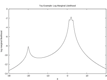
Figure 1. The log marginal likelihood of the toy example of sec-tion 4.1.
4.1. Toy Example. We consider first a toy example in one dimension for which we borrow example 1 of (Gaetan and Yao, 2003). The model consists of a Stu-dentt-distribution of unknown location parameterθwith 0.05 degrees of freedom. Four observations are available, y = (−20,1,2,3). The logarithm of the marginal likelihood in this instance is given by:
logp(y|θ) =−0.525
4 X
i=1
log 0.05 + (yi−θ)2
,
which is not susceptible to analytic maximisation. However, the global maximum is known to be located at 1.997, and local maxima exist at{−19.993,1.086,2.906}
as illustrated in figure 1. We can complete this model by considering the Student
t-distribution as a scale-mixture of Gaussians and associating a gamma-distributed latent precision parameterZi with each observation. The log likelihood is then:
logp(y, z|θ) =− 4 X
i=1
0.475 logzi+ 0.025zi+ 0.5zi(yi−θ)2
.
In the interest of simplicity, we make use of a linear temperature scale, γt=t,
which takes only integer values. We are able to evaluate the marginal likelihood function pointwise, and can sample from the conditional distributions:
πt(z1:t|θ, y) = t
Y
i=1 4 Y
j=1 Ga
zi,j
0.525,0.025 +(yj−θ)
2
2
,
(7)
πt(θ|z1:t) =N
θ µ
(θ)
t ,Σ
(θ)
t
,
N T Mean Std. Dev. Min Max
[image:10.595.118.409.292.371.2]50 15 1.992 0.014 1.952 2.033 100 15 1.997 0.013 1.973 2.038 20 30 1.958 0.177 1.094 2.038 50 30 1.997 0.008 1.983 2.011 100 30 1.997 0.007 1.983 2.011 20 60 1.998 0.015 1.911 2.022 50 60 1.997 0.005 1.988 2.008
Table 1. Simulation results for the toy problem. Each line sum-marises 50 simulations with N particles and final inverse temper-atureT. Only one simulation failed to find the correct mode.
where the parameters,
Σ(tθ)=
t
X
i=1 4 X
j=1
zi,j
−1
=
1/Σ (θ)
t−1+ 4 X
j=1
zt,j
−1
,
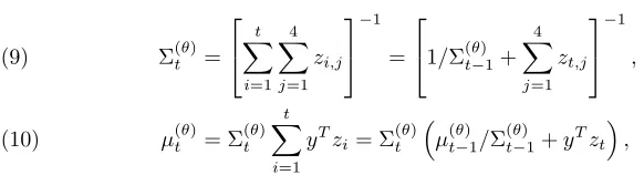
(9)
µ(tθ)= Σ
(θ)
t t
X
i=1
yTzi= Σ
(θ)
t
µ(t−θ)1/Σ (θ)
t−1+yTzt
,
(10)
may be obtained recursively. Consequently, we can make use of algorithm 3.1 to solve this problem. We use an instrumental uniform [−50,50] prior distribution over
θ. Some simulation results are given in table 1. The estimate is taken to be the first moment of the empirical distribution induced by the final particle ensemble.
This simple example confirms that the algorithm proposed above is able to lo-cate the global optimum, at least in the case of extremely simple distributions. It also illustrates that it is reasonably robust to the selection of the number of particles and intermediate distributions. Generally, increasing the total amount of computation leads to very slightly more accurate localisation of the mode. Only a single simulation failed to find the global optimum – one of those withN = 20 and
T = 30.
4.2. A Finite Gaussian Mixture Model. To allow comparison with other tech-niques, and to illustrate the strength of the method proposed here in avoiding local maxima, we consider a finite Gaussian Mixture model. A set of observations{yi}Pi=1
is assumed to consist of P i.i.d. samples from a distribution of the form:
(11) Yi∼
S
X
s=1
ωsN µs, σ2s
,
where 0 < ωs < 1; S
P
s=1
ωs = 1 are the weights of each mixture component and
{µs, σ2s}Ss=1is the set of their means and variances. As is usual with such mixtures,
it is convenient to introduce auxiliary allocation variables, Zi which allow us to
assign each observation to one of the mixture components, then we may write the distribution in the form:
Yi| {ω, µs, σ2s}, Zi=zi
∼ N µzi, σzi2
, p(Zi=zi) =ωzi.
1998). We consequently show the results of all algorithms adapted for MAP esti-mation by inclusion of diffuse proper priors (see, for example (Robert and Casella, 2004, p. 365)) , which are as follows:
ω∼ Di(δ)
σi2∼ IG
λ
i+ 3
2 ,
βi
2
µi|σi2∼ N αi, σ2i/λi
,
with δ,λi andβi are hyperparameters, whose values are given below.
It is straightforward to adjust our algorithm 3.1 to deal with the MAP, rather than ML case. For this application it is possible to sample from all of the necessary distributions, and to evaluate the marginal posterior pointwise and so we employ such an algorithm.
At iteration t of the algorithm, for each particle we sample the parameter es-timates, conditioned upon the previous values of the latent variables according to the conditional distributions:
ω∼ Di γt(δ−1) + 1 +n(⌊γt⌋) +γt♯∆n(⌈γt⌉), σ2
i ∼ IG(Ai, Bi) µi|σi2∼ N
γ
tλiαi+y(⌊γt⌋)i+γt♯∆y(⌈γt⌉)i γtλi+n(⌊γt⌋)i+γt♯∆n(⌈γt⌉)i
, σ
2
i
γtλi+n(⌊γt⌋)iγt♯∆n(⌈γt⌉)i
,
where we have defined the following quantities for convenience:
n(i)j=
i
X
l=1
P
X
p=1
Ij(Zl,p) ∆n(i)j=n(i)j−n(i−1)j
y(i)j=
i
X
l=1
P
X
p=1
Ij(Zl,p)yj ∆y(i)j=y(i)j−y((i−1))j
y2(i)
j= i
X
l=1
P
X
p=1
Ij(Zl,p)y2j ∆y2(i)j=y2(i)j−y2(i−1)j,
and the parameters for the inverse gamma distribution from which the variances are sampled from are:
Ai=
γt(λi+ 1) +n(⌊γt⌋)i+γt♯∆n(⌈γt⌉)i
2 + 1
Bi=
1 2
γt(βi+λiα2i) +y2(⌊γt⌋)i+γt♯∆y2(⌈γt⌉)i−
⌊γt⌋
X
g=1
(∆y(g)i+λiαi)2 λi+ ∆n(g)i
−γt♯
(∆y(⌈γt⌉)i+λiαi)2 λi+ ∆n(⌈γt⌉)i
.
Then we sample all of the allocation variables from the appropriate distributions, noting that this is equivalent to augmenting them with the new values and applying an MCMC move to those persisting from earlier iteration.
As a final remark, we note that it would be possible to use the proposed frame-work to infer the number of mixture components, as well as their parameters – by employing Dirichlet process mixtures, for example.
4.2.1. Simulated Data. We present results first from data simulated according to the model. 100 data were simulated from a distribution of the form of (11), with parameters ω= [0.2,0.3,0.5],µ= [0,2,3] andσ2=
1,14,161
N T χ Mean Std. Dev. Min Max
[image:12.595.160.435.118.215.2]25 25 1325 -154.39 0.55 -155.76 -153.64 25 50 2125 -153.88 0.13 -154.18 -153.59 50 50 4250 -153.80 0.08 -153.93 -153.64 100 50 8500 -153.74 0.07 -153.91 -153.59 250 50 21250 -153.70 0.07 -153.90 -153.54 1000 50 85000 -153.64 0.04 -153.71 -153.57 100 100 20300 -153.73 0.08 -153.92 -153.61
Table 2. Summary of the final log posterior estimated by 50 runs of the SMC Algorithm on simulated data from a finite Gaussian mixture with varying numbers of particles, N, and intermediate distributions,T.
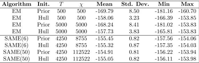
Algorithm Init. T χ Mean Std. Dev. Min Max
[image:12.595.125.472.292.403.2]EM Prior 500 500 -169.79 8.50 -181.16 -160.70 EM Hull 500 500 -158.06 3.23 -166.39 -153.85 EM Prior 5000 5000 -168.24 8.41 -181.02 -153.83 EM Hull 5000 5000 -157.73 3.83 -165.81 -153.83 SAME(6) Prior 4250 8755 -155.45 0.82 -157.56 -154.06 SAME(6) Hull 4250 8755 -155.32 0.87 -157.35 -154.03 SAME(50) Prior 4250 112522 -154.91 0.81 -156.22 -153.94 SAME(50) Hull 4250 112522 -155.05 0.82 -156.11 -153.98
Table 3. Performance of the EM and SAME Algorithm on sim-ulated data from a finite Gaussian mixture. Summary of the log posterior of the final estimates of 50 runs of each algorithm.
parameters was -155.87. Results for the SMC algorithm are shown in table 2 and for the other algorithms in table 3 – two different initialisation strategies were used for these algorithms, that described as “Prior” in which a parameter set was sampled from the prior distributions, and “Hull” in which the variances were set to unity, the mixture weights to one third and the means were sampled uniformly from the convex hull of the observations.
Two annealing schedules were used for the SAME algorithm: one involved keep-ing the number of replicates of the augmentation data fixed to one for the first half of the iterations and then increasing linearly to a final maximum value of 6; the other keeping it fixed to one for the first 250 iterations, and then increasing linearly to 50. The annealing schedule for the SMC algorithm was of the form
γt=Aebt for suitable constants to makeγ1= 0.01 andγT = 6. This is motivated
by the intuition that when γ is small, the effect of increasing it by some amount ∆γis to change its form somewhat more than would be the case for a substantially larger value of γ. No substantial changes were found for values of γ greater than 6, presumably due to the sharply peaked nature of the distribution. Varying the forms of the annealing schedules did not appear to substantially affect the results. Hyperparameter values were shared across all simulations, with δ = 1, λi = 0.1, βi= 0.1 andαi= 0.
Several points are noticeable from these results:
• The SMC algorithm produce estimates whose posterior density uniformly
N T χ Mean Std. Dev. Min Max
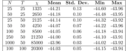
[image:13.595.163.428.119.227.2]25 25 1325 -44.21 0.13 -44.60 -43.96 50 25 2650 -44.18 0.10 -44.48 -43.95 25 50 2125 -44.14 0.10 -44.32 -43.92 50 50 4250 -44.07 0.07 -44.22 -43.96 100 50 8500 -44.05 0.06 -44.18 -43.94 250 50 21250 -44.00 0.05 -44.10 -43.91 1000 50 85000 -43.96 0.03 -44.02 -43.92 100 100 20300 -44.03 0.05 -44.15 -43.94
Table 4. Summary of the final log posterior estimated by 50 runs of the SMC Algorithm on the galaxy dataset of (Roeder, 1990) from a finite Gaussian mixture with varying numbers of particles,
N, and intermediate distributions,T.
the global optimum has been located it does provide some encouragement that the parameter estimates being obtained are sensible.
• For a given computational cost, the SMC algorithm outperformed SAME in the sense that both the mean and maximum posterior is substantially increased.
• Whilst, as is well documented, the EM algorithm can perform well if favourably initialised, neither of the initialisation strategies which we em-ployed led to a large number of good performances. Furthermore, it can be seen that taking the best result from 50 runs of the EM algorithm lead to poorer performance than a single run of the SMC algorithm with a lower cost:
– 50 runs of the EM algorithm with 500 iterations has cost slightly higher than a single run of the SMC algorithm withN = 250, T = 50 and the best result produced is significantly inferior to the poorest run seen in the SMC case;
– 50 runs of the EM algorithm with 5000 iterations has a cost more than 10 times that of the SMC algorithm with N = 250, T = 50 and the best result produced is comparable to the worst result obtained in the SMC case.
This provides us with a degree of confidence in the algorithms considered and their ability to perform well at the level of computational cost employed here, and the next step is to consider the performance of the various algorithms on a real data set.
4.2.2. Galaxy Data. We also applied these algorithms, with the same hyperparam-eters to the galaxy data of (Roeder, 1990). This data set consists of the velocities of 82 galaxies, and it has been suggested that it consists of a mixture of between 3 and 7 distinct components – for example, see (Roeder and Wasserman, 1997) and (Escobar and West, 1995). For our purposes we have estimated the parameters of a 3 component Gaussian mixture model from which we assume the data was drawn. Results for the SMC algorithm are shown in table 4 and for the other algorithms in table 5.
Algorithm Init. T χ Mean Std. Dev. Min Max
EM Hull 500 500 -46.54 2.92 -54.12 -44.32 EM Hull 5000 5000 -46.91 3.00 -56.68 -44.34 SAME(6) Hull 4250 8755 -45.18 0.54 -46.61 -44.17 SAME(50) Hull 4250 112522 -44.93 0.21 -45.52 -44.47
Table 5. Performance of the EM and SAME Algorithm on the galaxy data of (Roeder, 1990) from a finite Gaussian mixture. Summary of the log posterior of the final estimates of 50 runs of each algorithm.
performance (including the SMC algorithm) but these results illustrate that a rea-sonably straightforward implementation of the SMC algorithm is able to locate at least as good a solution as any of the other algorithms considered here, and that it can do so consistently.
4.3. Stochastic Volatility. In order to provide an illustration of the application of the proposed algorithm to a realistic optimisation problem in which the marginal likelihood is not available, we take this more complex example from (Jacquier et al., 2007). We consider the following model:
Zi=α+δZi−1+σuui Z1∼ N µ0, σ20
Yi= exp
Z
i
2
ǫi
where ui and ǫi are uncorrelated standard normal random variables, and θ =
(α, δ, σu). The marginal likelihood of interest, p(θ|y), where y = (y1, . . . , y500)
is a vector of 500 observations, is available only as a high dimensional integral over the latent variables,Z and this integral cannot be computed.
In this case we are unable to use algorithm 3.1, and employ a variant of algorithm 3.3. The serial nature of the observation sequence suggests introducing blocks of the latent variable at each time, rather than replicating the entire set at each iteration. This is motivated by the same considerations as the previously discussed sequence of distributions, but makes use of the structure of this particular model. Thus, at time t, given a set of M observations, we have a sample of ⌊M γt⌋ volatilities,
⌊γt⌋complete sets and⌊M(γt− ⌊γt⌋)⌋which comprise a partial estimate of another
replicate. That is, we use target distributions of this form:
pt(α, δ, σ, zt)∝p(α, δ, σ)
⌊γt⌋
Y
i=1
p(y, zt,i|α, δ, σ)
p
y1:M(γt−⌊γt⌋), z
1:M(γt−⌊γt⌋)
t,i
α, δ, σ
,
where z1:t,iM(γt−⌊γt⌋)denotes the first⌊M(γt− ⌊γt⌋)⌋volatilities of the ith replicate
at iterationt.
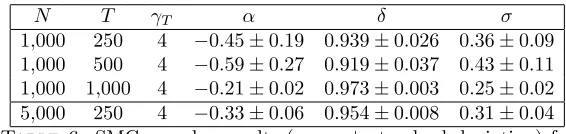
N T γT α δ σ
[image:15.595.154.437.117.184.2]1,000 250 4 −0.45±0.19 0.939±0.026 0.36±0.09 1,000 500 4 −0.59±0.27 0.919±0.037 0.43±0.11 1,000 1,000 4 −0.21±0.02 0.973±0.003 0.25±0.02 5,000 250 4 −0.33±0.06 0.954±0.008 0.31±0.04
Table 6. SMC sampler results (mean ±standard deviation) for simulated stochastic volatility data with generating parameters of
δ= 0.95,α=−0.363 andσ= 0.26.
4.3.1. Simulated Data. We consider a sequence of 500 observations generated from a stochastic volatility model with parameter values of δ= 0.95, α =−0.363 and
σ = 0.26 (suggested by (Jacquier et al., 2007) as being consistent with empirical estimates for financial equity return time series). The parametersµ0=−7, σ0= 1
were assumed known. Results are shown in table 6.
Note that a greater number of particles and intermediate distributions are re-quired in this case than were needed in the previous examples for a number of reasons. Unavailability of the likelihood makes the problem a little more difficult, but the principle complication is that it is now necessary to integrate out 500 con-tinuous valued latent variables.
The intention of this example is to show how the algorithm can be applied in more complex settings. The results shown here do not provide rigorous evidence that the algorithm is performing well, but heuristically that does appear to be the case. Estimated parameter values are close to their true values1 and the degree of dispersion is comparable to that observed by (Jacquier et al., 2007) at small values ofγusing data simulated with the same parameters. It can be seen that the results obtained are reasonably robust to variation in the number of particles and intermediate distributions which are utilised.
References
B. Amzal, F. Y. Bois, E. Parent, and C. P. Robert. Bayesian optimal design via interacting particle systems.Journal of the American Statistical Association, 101 (474):773–785, June 2006.
N. Chopin. Central limit theorem for sequential Monte Carlo methods and its ap-plications to Bayesian inference.Annals of Statistics, 32(6):2385–2411, December 2004.
P. Del Moral.Feynman-Kac formulae: genealogical and interacting particle systems with applications. Probability and Its Applications. Springer Verlag, New York, 2004.
P. Del Moral, A. Doucet, and A. Jasra. Sequential Monte Carlo samplers. Journal of the Royal Statistical Society B, 63(3):411–436, 2006.
A. P. Dempster, N. M. Laird, and D. B. Rubin. Maximum likelihood from incom-plete data via the EM Algorithm. Journal of the Royal Statistical Society, Series B, 39:2–38, 1977.
A. Doucet, N. de Freitas, and N. Gordon, editors. Sequential Monte Carlo Methods in Practice. Statistics for Engineering and Information Science. Springer Verlag, New York, 2001.
A. Doucet, S. J. Godsill, and C. P. Robert. Marginal maximum a posteriori esti-mation using Markov chain Monte Carlo. Statistics and Computing, 12:77–84, 2002.
A. Doucet, M. Briers, and S. S´en´ecal. Efficient block sampling strategies for sequen-tial Monte Carlo methods. Journal of Computational and Graphical Statistics, 15(3):693–711, 2006.
M. D. Escobar and M. West. Bayesian density estimation and inference using mixtures.Journal of the American Statistical Association, 90(430):577–588, June 1995.
C. Gaetan and J.-F. Yao. A multiple-imputation Metropolis version of the EM algorithm. Biometrika, 90(3):643–654, 2003.
C.-R. Hwang. Laplace’s method revisited: Weak convergence of probability mea-sures. The Annals of Probability, 8(6):1177–1182, December 1980.
E. Jacquier, M. Johannes, and N. Polson. MCMC maximum likelihood for latent state models. Journal of Econometrics, 137(2):615–640, April 2007.
A. M. Johansen. Some Non-Standard Sequential Monte Carlo Methods With Ap-plications. Ph.D. thesis, University of Cambridge Department of Engineering, 2006.
J. S. Liu and R. Chen. Sequential Monte Carlo methods for dynamic systems.
Journal of the American Statistical Association, 93(443):1032–1044, September 1998.
P. M¨uller, B. Sans´o, and M. de Iorio. Optimum Bayesian design by inhomogeneous Markov chain simulation. Journal of the American Statistical Association, 99: 788–798, 2004.
C. P. Robert and G. Casella. Monte Carlo Statistical Methods. Springer Verlag, New York, second edition, 2004.
C. P. Robert and D. M. Titterington. Reparameterization strategies for hidden Markov models and Bayesian approaches to maximum likelihood estimation. Sta-tistics and Computing, 8:145–158, 1998.
K. Roeder. Density estimation with cofidence sets exemplified by superclusters and voids in galaxies. Journal of the American Statistical Association, 85(411): 617–624, September 1990.
K. Roeder and L. Wasserman. Practical Bayesian density estimation using mixtures of normals. Journal of the American Statistical Association, 92(439):894–902, September 1997.
Adam M. Johansen – [email protected] – Department of Mathematics, University Walk, University of Bristol, Bristol, BS8 1TW, UK.
Arnaud Doucet – [email protected] – Department of Statistics & Department of Computer Science,University of British Columbia, Vancouver, Canada.