A Fault Injection Framework for Reliability Evaluation of Networks on Chip Designed for Space Applications

(1)

Faculty of Electrical Engineering,

Mathematics & Computer Science

A Fault Injection Framework for

Reliability Evaluation of

Networks on Chip Designed for

Space Applications

CONFIDENTIAL

Anindya Pakhira

M.Sc. Thesis

June 2016

Supervisors: Gerard Rauwerda

Recore Systems, Enschede, NL

Andr´e Kokkeler, Bert Molenkamp

(2)

(3)

Abstract

With the increasing complexity of circuits and decreasing feature sizes, it is becoming extremely difficult to manufacture fault-free circuits. Also, with the decreasing feature size comes a higher susceptibility to environmental factors like radiation. These fac-tors get compounded in a space context, where circuits are expected to have longer lifetimes and also be resistant to higher concentration of radiation from the free space. As a result, a lot of research has been conducted towards increasing the reliability and fault-tolerance of chips, in order to increase their lifetimes and resilience against errors. Processing requirements in space are also increasing, and many core processing is being introduced for space applications to address this trend. The huge amount of inter-core communication in these many core architectures necessitates networks-on-chip as the interconnect of choice. Network-on-Chips (NoCs) due to their complex nature are more susceptible to faults and failures. These two aspects necessitate the need for thorough investigation of the effects of faults in a space NoC context, in order to develop methods for detection and mitigation of the faults in the space environment .

In this context, a simulator for injecting different kinds of faults in a NoC has been developed. A SystemC based cycle-accurate simulator for NoCs called the NoC Explorer is already developed at Recore Systems. It has been extended with a fault injection framework that can inject transient as well as permanent faults at different locations of the NoC. A fault can be injected into six different components in or around each router of the NoC. The faults injected can be transient or permanent, the probability of which can be individually set by the user. The flits affected by the faults can be analyzed with the output files generated by the framework, which gives a great insight on how different faults can directly or indirectly affect the operation of a NoC in different conditions. In addition to this, Python scripts have also been developed, for generation of different statistics for the end user.

(4)

(5)

Acknowledgments

The decision to pursue my master’s education in a foreign country, leaving my job in India, was a big one on my part. However, in retrospect, it was the right decision which helped me pursue my dreams, and I have to thank my family and close friends back home for their support.

The research presented in this thesis has been done at Recore Systems, Enschede. I really want to thank Gerard, my supervisor at the company, for giving me the opportu-nity to pursue this topic in the company, and for his immense support and guidance. He has helped me along the whole way and has guided me when I have been stuck at prob-lems. I also want to thank Kim and all the others in the company who have provided me insight in different matters.

I would like to thank Andr´e and Bert, my supervisors from the Computer Architecture for Embedded Systems group in the University of Twente, for helping me regularly and guiding me towards the successful completion of my thesis. They have kept track of my progress and have helped me shape my thesis, giving me valuable and constructive feedback at every step of the way.

(6)

(7)

List of Figures

2.1. Network on Chip Topologies . . . 8

2.2. Turns in a Mesh or Torus . . . 10

2.3. Schematic of a router withnI/O ports and kinput VCs . . . 15

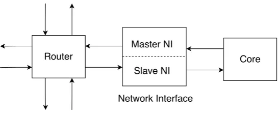
2.4. Network Interface . . . 16

3.1. Solar Flare [1] . . . 18

3.2. Coronal Mass Ejection [1] . . . 18

3.3. Fault Injection Techniques . . . 21

3.4. Types of Saboteurs . . . 23

4.1. NoC Explorer: Framework . . . 28

4.2. NoC Explorer: Router . . . 29

4.3. NoC Explorer: Master Network Interface . . . 30

4.4. Traffic Node Flowchart . . . 32

4.5. Data Flow for a Flit . . . 34

5.1. Router with Fault Injection Components . . . 40

5.2. Fault generation in physical links . . . 44

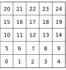
6.1. NoC Layout for Single Fault Testing . . . 48

6.2. Packet path for VC buffer test . . . 51

6.3. Packet path for flow control test . . . 53

6.4. Packet paths for RCU test . . . 55

6.5. Packet paths for Crossbars . . . 58

6.6. Packet paths for Physical Link & VC Allocator . . . 61

6.7. Literature Comparison for Transient Faults: VC Buffer Faults . . . 65

6.8. Literature Comparison for Transient Faults: Flow Control Faults . . . 66

6.9. Literature Comparison for Transient Faults: VC Allocator Priority Reg-ister Faults . . . 67

6.10. Literature Comparison for Permanent Faults: Throughput Degradation . 68 6.11. Literature Comparison for Permanent Faults: Delay Decrease . . . 69

(12)

(13)

List of Tables

2.1. Oblivious, Deterministic and Stochastic Routing Algorithms . . . 11

2.2. Adaptive Algorithms . . . 12

5.1. Effect of faulty components on OSI layers . . . 38

5.2. Flit Fault Probabilities . . . 43

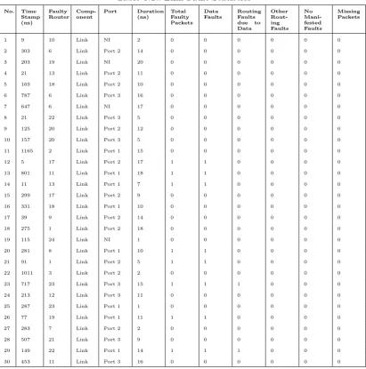
6.1. Link Fault Statistics . . . 49

6.2. VC Fault Statistics . . . 50

6.3. Flow Control Fault Statistics . . . 52

6.4. RCU Fault Statistics . . . 54

6.5. Crossbar Fault Statistics . . . 56

6.6. Physical Link and VC Allocator Fault Statistics . . . 60

6.7. Literature Comparison for Permanent Faults: Throughput . . . 68

6.8. Literature Comparison for Permanent Faults: Delay . . . 69

6.9. Callgrind Flat Profile for Original NoC Explorer . . . 71

6.10. Callgrind Flat Profile for NoC Explorer with Fault Injection — No errors inserted . . . 73

6.11. Callgrind Flat Profile for NoC Explorer with Fault Injection — Errors inserted . . . 74

(14)

(15)

Acronyms

CME Coronal Mass Ejection.

IC Integrated Circuit.

ITRS International Technology Roadmap for Semiconductors.

NBTI Negative Bias Temperature Instability.

NI Network Interface.

NoC Network-on-Chip.

OSI Open Systems Interconnect.

QoS Quality of Service.

RCU Routing Computation Unit.

SA Switch Allocation.

SDF Synchronous Data Flow.

SER Soft Error Rate.

SET Single Event Transient.

SEU Single Event Upset.

SoC System-on-a-Chip.

VA VC Allocation.

VC Virtual Channel.

(16)

(17)

Chapter 1.

Introduction

Reliability is a significant issue with all electronics systems, susceptible to aging and other transient effects [2]. With the advent of the nanoscale era, manufacturing reliable, completely fault-free, chips is becoming increasingly difficult and costly. As the technol-ogy scales, process variability leads to variability in transistor performance, making them gradually less reliable [3]. Rising complexity of circuits compounds the matter. This issue in reliability is not only restricted to manufacturing-time failures but also includes run-time soft errors and errors due to aging, the possibility of which also increases with technology scaling. The International Technology Roadmap for Semiconductors (ITRS) [4] identifies a long-term requirement for system-level reliability techniques for unreliable devices. All of these have led to significant research on designing fault-tolerant circuits with different methodologies.

The reliability problem is exacerbated in the space context[1] where both the aging and transient effects are more important. On the one hand circuits deployed in space need to be reliably functional for long periods of time in unmanned space locations, and on the other hand radiation effects from various phenomena like solar flares, cosmic rays, van Allen belts, etc. increase in space due to the absence of atmospheric protection. Hence there is a huge requirement for building reliable circuits for space. Traditionally reliability in space applications has been achieved by either of two methods. One is simply by using an older technology which is more resistant to radiation and aging. The other is by manufacturing circuits using radiation hardening processes, where the manufacturing process is modified in order to reduce the consequences of radiation. However the first method leads to more area and power requirements, and the second method is significantly cost intensive. Hence there is an interest in using software and digital logic solutions in current technology to enable reliable space applications.

1.1. Motivation

(18)

network like architecture, a NoC can support concurrent communication between pairs of nodes in the network and adapt to changing data transmission requirements. Hence SoCs for space are moving towards NoC interconnects.

A NoC constitutes the most area-intensive and complex subsystem in a many core architecture [8], and considering the high data throughput over long, high-capacity wires, it will lead to large heat dissipation. This accelerates the aging process of the circuit. This coupled with higher susceptibility to radiation and crosstalk effects imply a higher need for fault tolerant methods for NoCs. In order to effectively develop and evaluate methods for fault detection and mitigation in NoCs, as a first step, the effects of faults in the physical world on the functioning of a NoC need to be simulated and studied thoroughly. This can be done by developing a framework for fault simulation in a NoC, which can then be used to study the effects of faults in the NoC for different NoC application traffic and fault conditions. This can provide an understanding of which components of a NoC are more susceptible to errors due to faults, and thus are to be focused on more in regards to fault mitigation strategies. The simulation framework can later be used to test and evaluate the effectiveness of various fault detection and mitigation techniques.

1.2. Contribution

A SystemC based cycle-accurate simulator for NoCs has been developed at Recore Sys-tem, called the NoC Explorer [9]. In this thesis, an extension for the NoC Explorer is proposed which adds fault injection capabilities. A flexible fault injection framework is proposed, with user-definable parameters, for the insertion of faults into the NoC. Also written in SystemC and integrated into the NoC Explorer framework with suit-able modifications, it supports fault insertion into various components of the NoC and generates information about faults generated and NoC traffic affected by faults. Using Python scripts, this information is aggregated and converted into useful statistics and information for the end user.

A thorough analysis of the fault injection framework in action has been presented, with explanations of how a fault affects the NoC traffic directly as well as indirectly. A comparison of the fault injection framework with other methods used in the scientific community has been done, in order to compare and validate the functioning of the framework. Finally, the code has been profiled in terms of performance and compared with the performance profile of the original NoC Explorer, in order to quantify the performance overhead of adding the fault injection framework.

1.3. Outline

(19)

(20)

(21)

Chapter 2.

Networks on Chip: An Overview

In this chapter a general overview of NoCs is presented. First the need for NoCs in a modern many core architecture context is discussed and then the architecture of a generic NoC is touched upon. Next, the motivation for abstracting the NoC in terms of the Open Systems Interconnect (OSI) reference layers is explained. Finally NoC topologies, routing algorithms and flow control are discussed, ending with an explanation of the architecture of a router and network interface.

2.1. Bus Architectures and the Need for NoC

Inside a chip, the processing elements need to communicate with each other for comple-tion of the tasks as dictated by the applicacomple-tion. As more and more processing elements are packed into a chip, there is a greater need for efficient on-chip communication.

Traditionally on-chip communication in SoCs was based on point-to-point links and various interconnect architectures like simple bus, ring based bus, etc. [5]. As the number of cores and processing elements grew, problems started coming up with these intercon-nect architectures. With a high node count, point-to-point architectures, in which every node needs to be individually connected to the required nodes, become exceedingly com-plex and consume lots of power. In case of buses, the comcom-plexity is less of an issue, but the higher communication bandwidth requirement by multiple elements leads to bus contention, communication bottlenecks, arbitration issues and higher power usage [6, 7]. Hence bus architectures are not scalable for large, many-core systems.

Even though there is a large communication requirement between nodes in a many-core architecture, not all nodes need to be connected to every other node at any single point in time. Communication needs between nodes change throughout the application lifetime and at each point a node needs to be connected to a few nodes. There is thus a need for a “shared, segmented global communication structure [6]”, where each node can be connected to any node at will. This matches well with a data-networking architec-ture where individual data packets are routed between nodes as per the communication requirement. This idea has given rise to the notion of NoCs for many-core systems.

2.2. Introduction to NoCs

(22)

considered in the present work. The conversion of raw data from the processing nodes to packetized data is also handled by the NoC, making the communication transparent to the processing nodes. The main components of a NoC fabric are links, routers and

network interfaces.

Links They are the physical connection between routers, connected according to a

specific topology. They also connect the routers to the network interfaces. They can consist of one or more virtual or physical channels [6].

Routers They are responsible for routing the data from source to destination nodes

according to the specific routing protocol.

Network Interface (NI) It is the interface through which the processing core connects

to the router. It handles conversion of data from the core into packets and vice versa, essentially making communication transparent to the processing core.

The architecture of a router and an NI depends on some design criteria selected for a specific NoC, the concepts of which will be discussed in the following sections. After that, the architecture of the router and NI for our case will be discussed.

2.3. The OSI Model for NoC

Due to its architectural similarity with a computer data network, it has been considered that a NoC can be abstracted in terms of the Open Systems Interconnect (OSI) reference model [6]. For our purposes of the NoC the most pertinent layers are data link layer,

network layer and transport layer. The layer below the data link layer, the physical

layer is dependent on physical design of the circuit and is not concerned with the digital

design of the NoC. The higher layers are related to the software and middleware and hence not concerned with the NoC, with the assumption that the transport layer will provide reliable communication to the higher layers [8].

Data link layer is responsible for the reliable transmission and flow control of data

packets/flits through links [8]. In other words, it is responsible for the communication between pairs of routers, through the links. It consists of links, buffers and associated control signals and logic. The data link layer protocols work to improve reliability of the link, considering the physical layer to be not sufficiently reliable [10].

Network layer is responsible for the switching and routing of packets from the source

(23)

Transport layer is responsible for the end-to-end transmission of packets from source to destination nodes. This includes the whole path from a source network interface, through the different links in the path, to the destination network interface.

2.4. Topologies

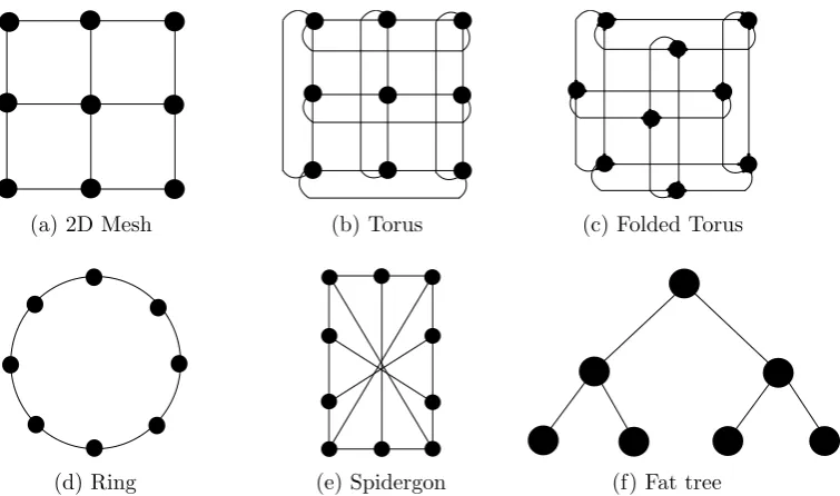
The NoC topology decides how the different nodes are physically connected to each other. It provides multiple paths for the movement of packets from source to destina-tion, in order to make the traffic uniform across the NoC. How the routing of packets takes place (i.e. the routing algorithm) is dependent on the topology selected. Different topologies exist suitable for different applications, like mesh, spidergon, ring, butterfly etc. They affect the network latency, throughput and power consumption. Hence a suitable topology must be carefully selected for the required application.

An informative way of expressing regular networking topologies is the k-ary n-cube,

n being the number of dimensions and k being the number of nodes in each of these dimensions [11, 12]. The number of nodes in ak-ary n-cube is given by [12]:

N =kn

In this present work we focus solely on two dimensional (2D) network topologies. Some of them are discussed below.

2D Mesh This is a k-ary 2-cube network, with bidirectional links, and is the topology

of choice for many NoCs. The nodes are arranged in a linear, equispaced array of two dimensions. Each node is connected to its 4 immediate neighbors except the edge nodes, which are disconnected in one or two directions.

Torus This is also a k-ary 2-cube network, with unidirectional links. They are arranged

similar to a mesh, except that the each edge node is connected to the opposite edge node, making the topology edge-symmetric. This property helps in balancing traffic load across the network and reduces the maximum number of hops by half, compared to mesh [9]. However due to the edge links, there are longer and more irregular delays in the network [6].

Folded Torus This is similar to the torus topology, except that a folding of the nodes

is employed to make the delays shorter and more uniform. Still, torus has longer delays than Mesh and hence is not preferred [6].

Ring A ring is like a torus, with k-ary 1-cubes. This is a simple topology in terms of routing. However it is not scalable since delays increase with increase of nodes.

Spidergon This has an even number of nodes, connected to neighbors, and also pairs

(24)

Fat tree It is a k-ary n-tree topology. It provides performance scalability (>64 cores) at the cost of higher power and area overheads [9].

(a) 2D Mesh (b) Torus (c) Folded Torus

[image:24.595.156.534.119.342.2]

(d) Ring (e) Spidergon (f) Fat tree

Figure 2.1.: Network on Chip Topologies

The aforementioned topologies have been shown in Figure 2.1. For the purpose of the present research, the topology chosen should be simple and efficient, for a moderate number of cores. Fat tree, with its high power and area costs, is not feasible for the moderate number of cores in the system. Spidergon has better performance than Mesh in some cases, but has more complexity and unequal lines. This makes routing algorithms more complicated and the latencies less predictable. This is not favorable for the design of fault tolerant algorithms. Mesh, in contrast, is simpler, with uniform latencies. Hence we would concentrate on Mesh topology for our research.

2.5. Routing

This section concerns with the path along which a packet is transferred from source to destination nodes across the network. Hence it works on the network layer. A routing algorithm is designed considering lowest latency and highest throughput for the system and application at hand [9].

2.5.1. Issues with Routing

(25)

Deadlock Deadlock refers to a cyclic dependency among nodes requiring access to common resources, due to which the packets in different nodes cannot make progress [13]. While certain routing algorithms are immune to deadlocks, they can be prevented by the use of virtual channels, among other techniques.

Livelock In this case packets travel around the network without ever reaching the

intended destination node [13].

Starvation Starvation refers to the phenomenon when a packet in a Virtual Channel

(VC) buffer cannot get access to an output channel in the network, or when a packet is not allowed to be injected into the network from an input buffer in a network inter-face. This happens when the output/input channel is always blocked by higher priority packets.

2.5.2. Routing Mode

This refers to the way packets are passed from one router to another inside the NoC. Alternatively called packet forwarding strategy, this is usually not dependent on the type of routing algorithm. The different routing modes are presented below:

Store-and-Forward Routing In this case each packet moves as a whole from one router

to the other. The entire packet is stored in the router memory before it is forwarded according to information contained in its header. Hence each buffer memory location must be as big as the largest possible packet according to the system design.

Wormhole Routing In this type of routing packets are divided into smaller units called

flits (flow control units) which then “worm” through the network. The first flit, called

the header flit contains the address information, and on the basis of this information

its next hop is determined and is immediately forwarded. The rest of the flits called

payload flits and tail flit follow the same path. Thus in a way this type of routing is a

combination of packet switching with the data streaming quality of circuit switching [6]. This leads to less latencies. However a stalled packet can cause all the links in the path to be occupied, which leads to more deadlocks. The main advantages are lower buffer memory requirement and lower latencies.

Virtual Cut Through Routing This has elements from both store-and-forward and

(26)

2.5.3. Routing Algorithms

Routing algorithms can broadly be divided in one way into deterministic, oblivious,

stochasticand adaptive [14]. This section concentrates on routing algorithms which are

either valid for all topologies or relevant to the mesh topology.

Deterministic They have specific, pre-determined paths for each source-destination

node pairs. They don’t change unless the network topology is changed. In congestion free networks they have low latency.

Oblivious These algorithms do not take into account network conditions like traffic

patterns, congestion, etc. They base their routing decisions on the basis of some fixed logic.

Stochastic As the name suggests, these algorithms make use of stochastic processes

to send packets. Multiple packets are sent out with random trajectories under the assumption that at least one will reach the intended destination. They are simple and inherently fault tolerant. However they lead to high network bandwidth usage.

Adaptive Adaptive routing algorithms intelligently adapt the routing paths to account

for changing network traffic conditions. However they are complex and take more re-sources to implement.

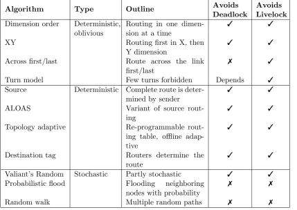
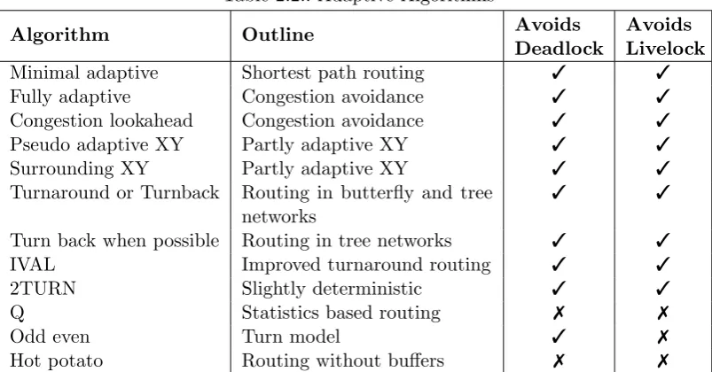
The different algorithms are summarized in a Tables 2.1 and 2.2, including information from [14]. Keeping in view the requirement for a logically simple routing algorithm, we are using XY Routing for our present work, which is explained below.

2.5.3.1. XY Routing

XY routing is a dimension-ordered, deterministic routing algorithm, which means that it routes at one direction at a time. Specifically, in XY routing, the packet is routed first through the X direction, and then through the Y direction, to reach its destination.

(a) All Turns (b) XY Turns

Figure 2.2.: Turns in a Mesh or Torus

(27)

[image:27.595.59.489.160.464.2]

move in any direction, as shown in Figure 2.2a. A deadlock occurs if a packet moves in a cyclic manner [15]. In XY routing this is preventing by forbidding two of the four turns, as shown in Figure 2.2b.

Table 2.1.: Oblivious, Deterministic and Stochastic Routing Algorithms

Algorithm Type Outline Avoids

Deadlock

Avoids Livelock

Dimension order Deterministic, oblivious

Routing in one dimen-sion at a time

3 3

XY Routing first in X, then

Y dimension

3 3

Across first/last Route across the link

first/last

7 3

Turn model Few turns forbidden Depends 3

Source Deterministic Complete route is deter-mined by sender

3 3

ALOAS Variant of source

rout-ing

3 3

Topology adaptive Re-programmable

rout-ing table, offline adap-tive

3 3

Destination tag Routers determine the

route

3 3

Valiant’s Random Stochastic Partly stochastic 3 3

Probabilistic flood Flooding neighboring

nodes with probability

7 7

Random walk Multiple random paths 7 7

2.6. Flow Control

Flow control concerns with how data flow is controlled from one router to another. Specifically, flow control determines how network resources like buffers are allocated to the different flits/packets and how competition of packets/flits for the same resources is resolved [16]. This is needed since the sending router (also known as upstream router) should only send the data when the receiving router (also known asdownstream router) is capable of receiving it. Flow control operates at the data link layer.

Some of the common flow control mechanisms are:

Credit based flow control In this method, an upstream router keeps track of available

(28)

[image:28.595.125.527.103.313.2]

Table 2.2.: Adaptive Algorithms

Algorithm Outline Avoids

Deadlock

Avoids Livelock

Minimal adaptive Shortest path routing 3 3

Fully adaptive Congestion avoidance 3 3

Congestion lookahead Congestion avoidance 3 3

Pseudo adaptive XY Partly adaptive XY 3 3

Surrounding XY Partly adaptive XY 3 3

Turnaround or Turnback Routing in butterfly and tree networks

3 3

Turn back when possible Routing in tree networks 3 3

IVAL Improved turnaround routing 3 3

2TURN Slightly deterministic 3 3

Q Statistics based routing 7 7

Odd even Turn model 3 7

Hot potato Routing without buffers 7 7

Handshake This is a simple mechanism where upstream router first asserts a VALID

signal after putting up valid data. The downstream router signals when it has received the correct data by asserting another VALID signal.

ACK/NACK This is similar to Handshake based flow control. However a copy of data

is kept in the sending router buffer until it receives the ACK signal from the receiving router. If the receivers detects the data to be incorrect or there is a timeout, it sends a NACK. If NACK is received the data is re-transmitted.

Besides this another concept that needs to be considered is virtual channel.

2.6.1. Virtual Channels

A VC is a logically separate channel by which a single physical channel can be shared by multiple flits/packets. This is specifically designed for wormhole type of routing and was first proposed by Dally [16]. Generally 2 to 16 VCs per physical channel are considered for NoCs [6].

At the heart of the VC concept are separate buffers for a single physical channel, corresponding to the separate VCs, along with the associated routing logic. Effectively, VCs allow a single physical link to be multiplexed, so that multiple packets can be transmitted during the same time frame, in a time-shared manner.

(29)

Network Interface The VC to be used is fixed at the source by the Master NI.

Dynamic The VC to be used is selected dynamically for each router, usually using a

round robin or priority based selection policy.

The main advantages of Virtual Channel based flow control are:

Deadlock avoidance Mutual independence from one VC to another means that

multi-ple packets can be in the process of transmission in the same physical channel, avoiding deadlock cases.

Performance improvement With multiple VCs, network performance is improved in

high load scenarios by preventing stalls.

Support for differentiated services VCs can be used to provide support for different

Quality of Service (QoS) for different channels. So data from higher priority VCs can overtake the data from lower priority ones.

The disadvantages of VCs are a higher power and area overhead due to control logic and duplication of buffers for each VC, and also latency overhead.

2.7. The Recore NoC

Recore has a packet-based NoC already developed for its multi core processing frame-work, which is planned to be extended with fault tolerance capabilities. Hence the present research will focus on simulating fault injection on a similar NoC. The main specifications of the Recore NoC pertaining to the present discussion are presented be-low:

• Packet based

• Wormhole based XY routing

• 4 service levels

• Credit based flow control

The service levels referred above are QoS levels, with level 0 being the highest priority and lowest latency, and vice versa for level 3. Hence, a packet with an assigned QoS level of 0 will be sent first through a link if it has a resource conflict with a packet with a lower priority level.

(30)

2.8. Representative NoC Architecture

In this section, the architecture of a router and the network interface, two of the primary components of a NoC, is explained. The architecture of routers could vary, depending on the required routing algorithm, flow control, etc. Hence a generic router which closely resembles the Recore NoC is detailed here.

2.8.1. Router

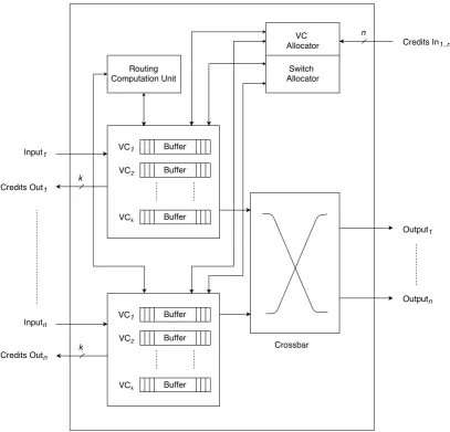
The routers are the main components in a NoC which are responsible for sending the packets along the correct links in order to reach the destination. The schematic of a generic router with credit based VC flow control is shown in Figure 2.3. The major components of the router are the VC buffers, Routing Computation Unit (RCU) , VC allocator, switch allocator and the crossbar. A thing to be noted is that although this router has been shown to have VC buffers only at the input side, some router designs have output VC buffers too, after the crossbar stage.

The routing steps undertaken by a generic router are as follows:

Routing Computation (RC) Based on the header flit information and the routing logic

selected, the RCU finds the output port to send the flits of the packet to.

VC Allocation (VA) The VC allocator checks the credits of the input VCs of the next

target router and, based on availability, assigns a VC to the current packet.

Switch Allocation (SA) The switch allocator selects which input port of the router

should be connected to which output port via the crossbar

Crossbar The crossbar then writes the flit to the correct output port.

These routing steps are usually pipelined, with each routing step corresponding to a pipeline stage. More efficient router designs sometimes combine one or more routing steps into a single pipeline stage, in order to reduce routing latency.

2.8.2. Network Interface

The Network Interface (NI) is the component which is responsible for communication between the processing core and the router in the NoC. It makes the communication between the two transparent. In other words the NI decouples the processing core from the NoC, facilitating the independent design of the two. The NI thus works at the Network Layer.

(31)

[image:31.595.60.468.81.472.2]

Figure 2.3.: Schematic of a router with nI/O ports andk input VCs

Master NI Master NI is the entity that initiates data transfer operations on the NoC.

It receives raw data from the processing core, packetizes it and sends it into the NoC. It is responsible for taking data and the address from the core, dividing it into suitable packets and flits, according to the network protocol, and sending it into the router.

Slave NI It receives flits from the network, correctly assembles them into packets,

depacketizes them into raw data. and then sends the raw data into the core.

(32)

[image:32.595.193.467.313.425.2]

(33)

Chapter 3.

Faults in Digital Systems

Before delving into how faults are modeled and simulated in the context of a NoC a discussion on the types of faults and how faults occur in nature should be looked into. Faults in digital systems can either be physical/hardware faults or faults in the software [17]. The present work focuses on the reliability evaluation techniques for a NoC and so the treatment is restricted to hardware faults. This chapter first discusses the broad classes of faults that can occur in a digital circuit and how they are actually manifested physically. Then the modeling of faults is discussed, and the concept of hierarchical fault modeling is introduced, which is of importance in developing fault injection methods for NoCs. Finally, different ways in which faults can be artificially injected into a system, in order to study their behavior, are discussed.

3.1. Fault Classes

Among the different ways to classify hardware faults in a digital system, a prevalent way is to classify them based on frequency of occurrence, into transient, intermittent and

permanent faults [18].

Transient Faults These faults happen randomly, usually in response to phenomena like

external radiation, crosstalk between wires, etc. The rate of occurrence of these faults remains constant on average during the lifetime of a chip. The errors that result from transient faults are known as transient errors, or alternatively, soft errors.

Intermittent Faults They are very similar to transient faults when a single fault

oc-currence is viewed separately. However, according to [18] the distinguishing criteria are repetitive occurrence in a single location, a tendency to occur in bursts and the problem being solved when the “offending circuit” is replaced.

Permanent Faults These faults, when they manifest, remain for the rest of the lifetime

(34)

3.2. Fault Generation Mechanisms

MOSFET-based circuits, which are the most prevalent type of circuits currently in pro-duction, can face erroneous behavior due to device physics and materials, mainly from radiation, electromagnetic interference, electrostatic discharge and aging [8]. They cause one or more of the classes of faults discussed in the previous section.

3.2.1. Radiation

System failure due to radiation is one of the biggest issues for electronics systems both for space and ground applications [1]. The effect of radiation is greater in the space context because of the lack of atmospheric protection. The sources of these are mainly radiation from space as well as alpha particles that are generated from radioactive impurities inside the devices and their packaging [8]. Atmospheric radiation sources could be from the sun or from outside the solar system [19], which could be caused by solar flares [Figure 3.1], Coronal Mass Ejections (CMEs) [Figure 3.2], solar winds or galactic cosmic rays.

In terms of their effect on electronic circuits, these radiations cause one or more logic values to invert in the circuit. When the bit flip occurs in a memory cell, it is called a

Single Event Upset (SEU), and when it causes an inversion of voltage levels in a wire or

logic gate, it is known asSingle Event Transient (SET)[8]. These are both examples of

transient faults.

The probability of an SEU occurring depends on the critical charge needed for a bit flip [8]. This required critical charge decreases with technology scaling, and hence SEU probability increases with newer technology. In fact the Soft Error Rate (SER) due to radiation increases by 8% per memory cell with every technology generation [20]. This, coupled with the fact that more bits/memory cells are incorporated into a chip with newer technology, means that the effect of radiation increases significantly with each technology generation. The error rates in case of SET in wires and combinational logic also grows at a similar rate [21, 22] but are masked since they only manifest when they get latched at clock edges, resulting in lower effective error frequency.

[image:34.595.387.482.567.655.2]

Prolonged exposure to radiation over a course of years can also lead to permanent faults in the circuits. The methods for handling these faults are different from those for transient faults.

[image:34.595.179.268.569.654.2]

(35)

3.2.2. Electromagnetic Interference

Electromagnetic interference is primarily caused due to crosstalk between long wires [8]. As technology scales, wires become thinner and hence resistance becomes higher. To counteract this, wires are made taller, resulting in higher coupling capacitance and inductance between parallel wires. This leads to delays, glitches and damped voltage variations [23]. Another problem is the Skin Effect [24] with wires carrying high fre-quency signals which causes wire resistance to be frefre-quency-dependent. This leads to signal delays in turn being dependent on frequency [25].

3.2.3. Electrostatic Discharge

A sudden discharge of electricity through an electronic device can cause its breakdown [8]. This current can be flowing in through an input pin or be induced from external fields. However in modern ICs protection from electrostatic discharge is usually incorporated in the I/O pins and circuit.

3.2.4. Aging

Aging is one of the major causes of errors in electronic circuits which finally leads to permanent faults. There are various aging-related effects which cause degradation of the circuit over time:

Electromigration is the transport of metal atoms in wires induced by high current

density. It thus thins out the wear, causing even higher current density and hence aggravating the process. Initially it causes increasing delay and eventually an open circuit between previously connected wires or short between previously open wires [18].

Negative Bias Temperature Instability (NBTI) is the gradual increase of threshold

voltage of a MOSFET and the consequent decrease in drain current, due to the migration of charge into the gate oxide. It is very sensitive to temperature increase but the effect slows down with higher signal frequency [26].

Hot Carrier Injection has an effect similar to NBTI. In this phenomenon fast

carri-ers (electrons/holes) are injected from the conducting channel into the insulating gate dielectric, made of Silicon Dioxide (SiO2). The threshold voltage increases and hence

degrades speed of operation [27].

3.3. Fault Modeling

(36)

different parameters, to closely model real world fault conditions. However, transient and permanent faults are in general modeled with some basic characteristics which are explained below:

3.3.1. Transient Fault Modeling

The basic units with which transient faults can be modeled are SETs and SEUs. As discussed previously. an SET occurs when an energy pulse is issued from the ionization of a component in an electronic circuit by radiation, leading to an inverted logic transient [1]. An SEU occurs when radiation similarly affects a storage element like a flip-flop, latch, SRAM cell, etc., leading to the error being present till a new value is written into the storage element. An SEU can also occur by an SET being latched on a clock edge into a storage element.

An SET can be modeled as a bit flip in a signal, and SEU as a bit flip in a register or memory cell [28]. In the case of an SET being latched into a storage element, the effects can be modeled by directly considering it as an SEU in most cases, since these would be synchronous circuit elements. The parameters concerned with a transient fault occurring in a particular component are the transient fault error rate or transient fault probability, as well as the duration.

3.3.2. Permanent Fault Modeling

Permanent faults can occur in the form of logic faults and delay faults. How they are modeled also depends on the component that is being modeled. Logic faults in memory devices can be stuck-at faults, where certain bits in a memory cell are stuck at a high or low value, respectively called a stuck-at-1 or stuck-at-0 fault. Faults in wires can be broken wires, which can be modeled as stuck-at-0 faults at the inputs to components. Wires can also be short-circuited to another wire, which is known as a bridging fault. This is modeled by mirroring the signal in the faulty wire with that of another wire. A special case of this is when the wire gets shorted to a power supply rail or a ground plane, which can be modeled as stuck-at-1 and stuck-at-0 respectively.

Since permanent faults occur with lower probability than transient faults [29], a sep-arate permanent fault probability value is usually used to model the frequency of occur-rence of such faults.

3.3.3. Hierarchical Fault Modeling

(37)

In later chapters where fault modeling of a NoC is considered, it will be seen that the NoC faults can best be hierarchically modeled following the OSI layer model.

3.4. Fault Injection

Fault injection is the artificial insertion of faults into a system, in order to observe the resulting behavior [17]. The effects of faults on system performance can be analyzed, which is then used to evaluate a system’s resilience to faults and also to validate fault detection and mitigation mechanisms.

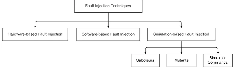
Fault injection systems can be designed for both electronic hardware and software systems to evaluate their respective fault resilience. There are various ways by which faults can be injected, depending on the requirements. A classification of the broad types have been given in Figure 3.3.

3.4.1. Hardware-based Fault Injection

Hardware-based fault injection involves directly exercising the system under considera-tion with faults injected with the help of special test hardware [17]. Usually the faults in this case are injected at the Integrated Circuit (IC) pin level, but some designs exist where the faults are injected internally into the chip.

Advantages of this method are higher fault location coverage in some cases, real-time and high resolution fault injection, leading to fast and accurate experiments. Finally, the fault injection is done on real hardware and software and hence takes into account the most realistic possible depiction of the system, without requiring any modeling or validation.

However this method has its disadvantages. Externally forcing faults can cause damage to the circuit. Location and types of faults that can be injected are limited, along with low observability of the fault effects, due to the access to the system through external pins only. Also, hardware-based injection requires specific hardware for each system to be injected with faults, leading to low portability and high initial setup time and cost.

[image:37.595.72.460.542.659.2]

In the present work, we need high observability and control over fault injection, so that effects of faults on individual flits/packets can be observed. Also, the objective is

(38)

more of a design space exploration instead of benchmarking a fully developed system against faults. Hence this method is not suitable for our case.

3.4.2. Software-based Fault Injection

This is a software-driven way of injecting faults into a complete hardware/software sys-tem. The faults are injected to simulate faults occurring in the system and it can be used to inject various kinds of faults, from memory faults to network errors and erroneous program flags [17].

Advantages are the ability to inspect faults in software which is not possible in hard-ware based fault injection, and running the injection on real hardhard-ware, requiring no model development. At the same time, it does not require extra hardware, so set up cost is low.

Disadvantages are that injection location and timings are less flexible, and certain hardware faults cannot be simulated and/or observed from the software level. Also, it requires modification of the original software, which might lead to performance changes and also affect scheduling in time-critical applications.

In our present work, the NoC is a fully hardware centric system and hence software based simulation methods are not applicable. On higher layers of abstraction, when the NoC is used in practice with the Recore multi-core framework, software based fault injection method may be used to access and evaluate certain areas of the system.

3.4.3. Simulation-based Fault Injection

This involves the creation of a model of the entire system under consideration and adding fault injection into the model. The simulation models were traditionally specified using a hardware description language like Very High Speed Integrated Circuit Hardware Description Language (VHDL) or Verilog, like the MEFISTO [30] tool. However recently the same concepts have been translated into SystemC models [31]. SystemC, being able to simulate more complex systems faster and at higher abstraction levels, is considered to be useful in fault injection of large complex systems. In case of simulation based fault injection methods an important consideration is the accuracy of the model and determining what level of accuracy is actually needed for the application at hand.

Advantages are huge flexibility, in terms of fault models and injection, and support for any level of abstraction, depending on the model. It affords maximum controllability and observability, at the same time needing no extra hardware [17].

The disadvantages are all related to modeling, which requires lots of development efforts. Also, the accuracy of the model directly relates to how accurate the fault injection system would be.

Since we are targeting a fault injection tool which will help in evaluation of fault tolerance techniques in a high abstraction level, simulation-based fault injection suits our purposes well.

(39)

(a) Serial Simple _{(b) Serial Complex}

(c) Parallel

Figure 3.4.: Types of Saboteurs

either a saboteur or mutant, which pertain to structural or behavioral features of the model, respectively [17]. Another method, using simulator commands, does not require the modification of the hardware description.

3.4.3.1. Saboteurs

A saboteur is a special component added to the original model in between a signal to modify its data or timing characteristics [17]. It is activated when an external control signal is asserted, otherwise it passes on the data unmodified.

Saboteurs can be of three main types [17]:

Serial Simple Saboteur It intercepts a signal from a source to a destination port and

modifies it.

Serial Complex Saboteur It intercepts the signals between two or more sources and

destinations and modifies their signals according to some complex fault model. It can be used to model crosstalk [32] or bridging faults between signals for example.

Parallel Saboteur In this case no signal path is broken. It is added as an additional

driver for a resolved signal [30]. It is useful for simulating disturbances on buses [32].

Saboteurs are relatively easier to implement but are limited to only modeling faults in signals. Hence they are used in simple cases. The different types of saboteurs are shown in Figure 3.4.

3.4.3.2. Mutants

(40)

3.4.3.3. Simulator Commands

This technique involves using the commands of the simulator to inject faults at simulation time [17]. Since the built in commands of the simulator are used, there is no requirement for modifying the original model in any way, making this a very non-intrusive fault injection method.

(41)

Chapter 4.

NoC Simulation Tools

For quick benchmarking and evaluation of a system, developing a simulation platform which emulates the behavior of the original system is beneficial. This chapter discusses some openly available simulation tools for NoCs and then pertinent details of the NoC Explorer that has been developed in-house at Recore Systems.

4.1. NoC Simulation Tools

There have already been some simulation tools developed for NoC both in academia and industry. They support different subsets of features, and have been written using different languages. A brief overview of some of the common and popular tools is given below.

4.1.1. BookSim

BookSim [34, 35], a product of Stanford University, is one of the most widely used NoC simulators currently available. It is a highly detailed, modular, cycle accurate simulator written in C++ and can also be used for simulating other kinds of networks besides NoCs. Due to its flexible and modular nature, it can be modified in diverse ways to emulate many network configurations. In terms of configuration, the current version (BookSim 2) supports 8 standard topologies along with user-specified topology, standard and custom routing functions, and virtual channels with customizable buffer size. Many other functions and components are customizable like the switch allocator, VC allocator, etc. It supports both open-loop and closed-loop synthetic traffic generation and can be interfaced with a full-system simulator to use its traffic. It does not support power-area analysis and mixed language simulation.

4.1.2. NoCsim

(42)

4.1.3. Noxim

Noxim [38] is another SystemC based NoC simulator developed at University of Catania, Italy. It only supports 2D mesh topology with wormhole routing. Network size, buffer size, packet size, routing algorithm, traffic pattern etc. can be configured. There is no support for custom traffic. Results are in terms of throughput, average and maximum latency, received packets and flits, total energy consumption. In addition, the work done by each system element and detailed activity of flits can be seen. Area-power analysis and mixed language simulation is not supported. Recently Noxim has been extended [39] to support simulation of Wireless NoC (WiNoC) architectures in addition to conventional wired NoCs.

4.1.4. NoCTweak

NoCTweak [40, 41] is also another SystemC based NoC simulator developed at UC Davis. The currently available version supports 2D mesh topology, with customizable parameters like routing algorithm, virtual channels, buffer depth, switch arbitration, etc. Traffic can be synthetic or real embedded application traces input from files. It also has power and area models from commercial processes. Results generated are parameters like throughput, latency, power and energy consumption.

Although each one of these simulators have their own strengths, most of them are not suited for simulation of faults in the NoC. Booksim, being a highly modular simulator, can be extended to support fault injection, as done in [42] for example. However, it does not support mixed-language simulation, which helps in simulating NoC hardware more realistically. Noxim has also been used for fault injection, for example in [43], but also cannot support mixed-language simulation. In addition, it only supports the mesh topology and has no support for custom traffic scenarios. Thus there is a need for a NoC simulator with fault injection which has support for multiple topologies and algorithms, and mixed-language simulation. The NoC Explorer has all of these features, and in addition, it has now been extended to show detailed activity of flits and packets (explained in Section 5.2.1.6) like Noxim. Hence it is deemed to be a suitable candidate for a fault injection framework.

In this context it should be noted that though the simulation and testing in Chapter 6 is focused on NoC with a 2D mesh based topology and wormhole based XY routing, as explained in Section 2.4, the fault injection framework designed in this present work is compatible with other NoC topologies and schemes as well.

4.2. NoC Explorer Features

(43)

support for fault injection capabilities in the design space exploration. The extended NoC Explorer could possibly be used to find out the effectiveness of various techniques for fault tolerance at different components of the NoC, which would facilitate the design of a final fault tolerance NoC product in the future. A brief idea about some of the aspects of the NoC Explorer, which relate to the fault injection system, are discussed next.

4.2.1. Configuration and Simulation

• Topology: Support for mesh, torus, folded torus and spidergon topologies. More

topologies can be supported if designers add more custom modules.

• Routing Algorithm: XY routing for mesh topology, Torus XY for torus topology,

routing across first or last for spidergon topology.

• Network Size: Number of routers for X, Y direction in case of mesh based

topologies, and number of nodes for spidergon topology.

• Virtual Channels: VCs can be configured on the basis of number of VCs, buffer

depth and VC allocator and arbiter policies.

• Clock: Supports different clock frequencies for NoC.

• Mixed Language Simulation: Modules within the NoC simulator can be

re-placed with VHDL modules, supported by simulators like Questasim, which would provide more accurate RTL level simulation instead of Transaction Level from SystemC.

4.2.2. Traffic Generator

The traffic generator of NoC Explorer supports:

• Synthetic and Custom Traffic

• Flit Interval Selection

• Simulation time parameters 4.2.3. Results

NoC Explorer generates CSV data about flits. This is aggregated by the Python scripts to generate useful data.

4.3. NoC Explorer Framework

(44)

4.3.1. SystemC Modules

The hierarchy of the SystemC modules in the NoCExplorer is shown in Figure 4.1, taken from [9]. It has three main components: the NoC library, the traffic generator and the traffic manager. These are discussed, followed by an overview of the packet and flit format that has been used.

Figure 4.1.: NoC Explorer: Framework

4.3.1.1. NoC Library

This consists of SystemC descriptions of routers, network interfaces, packet and flit modeling and the network topology containing all of these components. The NoC library is described in hierarchical SystemC modules, the description of which follows:

Topology This decides the topology in which the whole NoC will be laid out, as

spec-ified by the user. Depending on user input, it instantiates a number of routers and corresponding network interfaces, and connects the data and control signals according to the specified topology.

Router This is a hierarchical implementation of the router component. It is divided into

separate SystemC modules, comprising of RCUs, VCs, physical link and VC allocator and crossbar. The RCU and the VCs are instantiated as many times as there are input ports in the router. The crossbar and the physical link and VC allocator are each instantiated once. The data and control paths of the router for one input port are shown in Figure 4.2.

(45)

Figure 4.2.: NoC Explorer: Router

sent to, using the routing algorithm specified by the user. It then writes this output port direction information into all the flits in the flit packet and writes them into the correct VC as specified in the VC field of the flits.

The VC component implements a set of FIFO buffers for VCs, and also contains logic for flow control. There is one input port and multiple outputs corresponding to the physical outputs of the VCs to the next stage. It reads in the flit sent by the RCU, and based on the VC write select signal, writes it into the correct FIFO buffer. In accordance with the wormhole routing protocol, it sends an acknowledgment signal (ACK) after the Tail flit is written, signaling the end of reception of the packet to the upstream router/NI. The VC component also maintains the flow control credit counters and sends the available credit information about every VC to the upstream router/NI.

The Physical Link and VC Allocator corresponds to the VA and SA stages of the

router. It performs the following steps:

1. Read the flits from the VCs of all the output ports, in the priority decided by the physical input port arbiter and the VC arbiter (can be round robin or priority based, as selected by the user).

2. If it is a Head flit:

a) From the output direction calculated by RCU, find the output port (physical link to be used).

b) Select a VC which is free on the next stage router according to user-specified VC selection policy (could be dynamically chosen or could be the VC chosen by the network interface). Wait if VC is not free.

c) Enable the appropriate signal in the crossbar so that the input port to output port connection is enabled.

3. Check for free credits and keep on sending flits from the input port to the output port.

4. If it is a Tail flit, write the flit to the output port and close the connection.

Thecrossbar is like a matrix which connects a specific input stage to an output port.

(46)

that each input port can be connected to all the output ports, including the output port associated with its own direction. This means a flit can enter a router and be returned back to the upstream router.

Network Interface The NI serves as a bridge between a node and a router, and is

required to support bidirectional communication, i.e. transmission and reception of packets. Hence it can be divided into two main components, viz. the Master NI and the Slave NI, which have been defined separately in the NoC Explorer. In essence the NI is to be designed in such a way that to the router it looks like another generic router, and to the node it looks like a generic memory location.

Figure 4.3.: NoC Explorer: Master Network Interface

A schematic of the Master NI is shown in Figure 4.3. In the Master NI there are two arbiters for VCs, one for input and the other for output. The VC output arbiter monitors the credits available in the VCs of the router and sends flits to the router accordingly. The VC input arbiter determines which VC the incoming data from the node is to be stored.

Since the node is oblivious to credit availability, the VC input arbiter just sends a signal which informs the node if there is any free VCs available. When a free VC is available, the node sends the packet request, which is then converted into packets and flits by the packet and flit assembler. The VC input arbiter then stores it into a VC based on the VC allocation scheme set by the user. Based on the credit availability in the connected router and the VC arbitration scheme, the VC output arbiter transmits the flits to the router. The rate at which a flit is written into the VC can be set by the flit interval selection mode.

The Slave NI functions in a similar way. It receives flits from the associated router, following flow control and VC arbitration policies, and assembles them into packets. Since this is a simulator, the disassembly of packets into raw data has been omitted since the node does not use received data in any way.

4.3.1.2. Traffic Generator

(47)

has support for both synthetic traffic as well as custom traffic specified by Synchronous Data Flow (SDF) graphs.

The main functional component of the traffic generator is the traffic node. The NoC Explorer can be used to model nodes, one of which can be connected to a single NI. To specify the characteristics of each node, the following parameters can be set by the user:

Destination Node Selection The destination node can be randomized for synthetic

traf-fic or be fixed for user defined custom traftraf-fic. The possible options are random, fixed, neighboring, transpose and round robin neighbor destination node.

Data Size This, in conjunction with the data width of each flit, determines the packet

size, or the number of flits in a packet.

Operational Limits A node can be started and/or stopped based on certain parameters.

A start time can be set. The node can also be stopped based on end time, a data limit, or after sending a specific number of packets into the network.

Bandwidth The bandwidth parameter is used to determine the flit injection rate, which

is the rate at which new flits are injected from the node into the network.

Internal Memory Internal buffer memory can be specified to model specific application

scenarios.

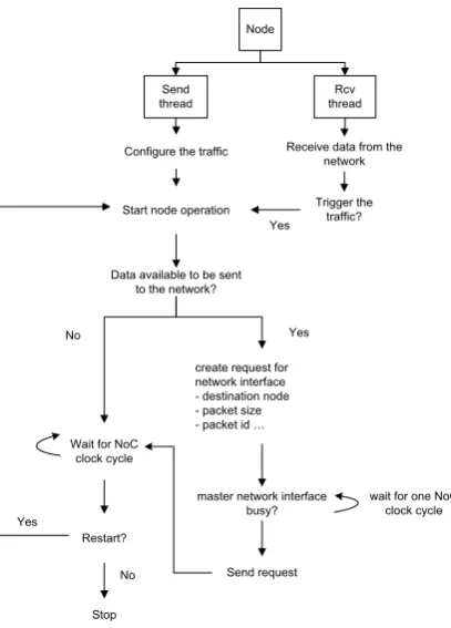
The node is implemented using two primary threads, asend threadand areceive thread. Based on the node modeling parameters, thesend thread requests a data transfer to the Master NI and sends the data, which is then packetized and sent into the network by the Master NI. The receive thread coordinates the reception of data from the Slave NI. A flow chart of how the node is modeled using the two threads is shown in Figure 4.4, taken from [9].

4.3.1.3. Traffic Manager

The traffic manager receives incoming packets (to the destination node) from the NoC through the Slave Network Interface and monitors the data. It is a single component which is connected to the output of every slave NIs in the network. It is responsible for time-stamping each flit as it leaves the network, and also to check out of order arrival of flits.

In addition, it writes a set of output files regarding the traffic and the NoC resources:

trafficPattern.csv This contains information about the packets that are accepted into

the NoC.

outputFlit.csv This file stores information about the flits which leave the NoC after

(48)

Node

Send thread

Rcv thread Configure the traffic

Start node operation

Data available to be sent to the network?

Wait for NoC clock cycle

Restart?

create request for network interface - destination node - packet size - packet id …

master network interface busy?

wait for one NoC clock cycle

Send request

[image:48.595.230.434.81.365.2]

Receive data from the network Trigger the traffic? Yes Yes Stop No Yes No

Figure 4.4.: Traffic Node Flowchart

noConfig.csv This stores the configuration of the NoC in the current simulation run.

routerCongestion.csv The router performance and any bottlenecks can be determined

from this file, which stores the average number of flits per cycle that each router has processed.

linkUtilization.csv This file stores information about link bottlenecks and performance.

4.3.1.4. Packet and Flit Format

Since the Noc Explorer uses wormhole type of routing, the packets are divided into separate flits, which are re-assembled at the destination. In the NoC Explorer, a flit is transmitted in the form of a System C data structure containing the following data fields:

Flit type Head, Body or Tail type of flit.

Flit sequence number This is the order in which the flits of a packet are sent, so that

they might be re-assembled in the correct order at the destination.

(49)

VC Number The VC to be used by all the flits of the packet while traversing a specific router.

Output port direction This is updated by the RCU of each router, which is then used

by the physical link and VC allocator to send the correct signal to the crossbar.

Source and Destination nodes The information is used by the routing logic only in the

case of the Head flits, since the simulator uses wormhole routing. In case of other flit types, this is only for post-simulation analysis.

Packet ID Each packet is given a unique ID for diagnostic and analysis purposes.

Hop count Used for performance evaluation of routing algorithms for a specific

appli-cation scenario.

Timestamps Entry and exit timestamps are recorded for performance and latency

mea-surement.

4.3.2. Python Scripts

NoC Explorer provides with multiple Python scripts for post-simulation analysis of the NoC performance. A description of the different python scripts in NoC Explorer along with their usage is given in Appendix B.

Missing Flits Using the traffic pattern and the output flit information, the flits that

are missing can be found out. That could be because of deadlock, insufficient simulation time or other faults generated in the NoC by the fault injector.

Latency and Throughput Analysis Various statistics about the NoC traffic like accepted

and ejected loads/cycle, VC utilization, packet and flit latency is provided.

Heat Map This provides a map of router and link utilization in the selected topology.

4.4. Data Flow

It is helpful to understand the data flow as a flit starts from its source and reaches its destination, in order to to better understand where and how faults can be injected. A broad overview of how a flit moves from source to destination is presented below, which is also represented in Figure 4.5, taken from [9].

1. Traffic node generates data and sends it to the Master NI

2. The Master NI divides this data into packets and flits, determines a VC to be used and stores the flits into the VC.

(50)

Synthetic traffic Custom / SDF based traffic Node Packet and flit assembly Master network interface Virtual channel Flow control Slave network interface Virtual channel Flow control Router Flow control Flow control Route compute Virtual channel Physical link and virtual channel allocation Crossbar Traffic manager Output analysis files Traffic generator

and manager Network Interface Router

Index Data flow Control signal flow Buffers

Figure 4.5.: Data Flow for a Flit

4. The RCU determines the output port to send the flits to, according to the routing algorithm, and writes that information into the flit. It then writes the flits into the correct VC.

5. The physical link and VC allocator eventually reads the flits and determines the VC to be used for the next router. It writes this information into the flit and signals the crossbar to send the flit to the specific output port.

6. The crossbar writes the flit to the correct output port.

7. On reaching the destination router, the flit is sent to the Slave NI

8. The Slave NI reassembles the flits into packets in the correct order.

(51)

Chapter 5.

Fault Injection in the NoC Explorer

This chapter concerns with the design and implementation of the fault injection frame-work for the NoC Explorer. Before delving into the specific design aspects, it is beneficial to discuss the faults that need to be simulated in terms of function and location, in or-der to model them correctly. Hence the first part of the chapter puts forward the ways that faults can be classified and modeled, and discusses the best way to work with when it comes to building a fault injection framework. The second part then explains the specifics of the fault injection framework that has been implemented for the NoC Explorer.

5.1. Modeling and Classification of Faults

The faults in different components of a NoC can be looked at from two different per-spectives: a physical location perspective, or from a functional perspective in terms of OSI layers. Radetzki et al. [8] and Wuderlich et al. [44] give a detailed account of fault classification and modeling in terms of OSI layers. The OSI layer model helps in un-derstanding how faults affect the system and give an idea of what broad ways to tackle the problem. However, faults can also be distinguished in physical location terms, into faults in the control logic and datapath [45].