Spherical harmonics based aggregation in the multilevel fast multipole algorithm MSc Thesis

(1)

NLR-TR-NLR-TR-2015-218

Spherical harmonics based aggregation in the

multilevel fast multipole algorithm

MSc Thesis

S. Hack

No part of this report may be reproduced and/or disclosed, in any form or by any means, without the prior written permission of the owner.

Customer NLR

Contract number

----Owner NLR

Division Aerospace Vehicles Distribution

Classification of title Unclassified June 2015 Approved by:

(2)

(3)

computations. In a simplified model, the scatterer is seen as a conductor, with an electric field that is zero inside. An incident radar wave induces a fictitious current on the surface of the scat-terer, which cancels the incident wave. The current satisfies a boundary integral equation, which is derived from the Maxwell equations.

Discretization using the boundary element method results in a dense system matrix, because every pair of basis functions interacts through the Green’s function for the vector Helmholtz equation. The system matrix is too large even to be stored in the computer’s memory for real-istic radar frequencies. In 1987, Rokhlin and Greengard proposed the fast multipole method (FMM) [15], which has been named as one of the top ten algorithms of the twentieth century [10]. The matrix-vector products in the Krylov subspace iterations are computed with complex-ityO(NlogN), rather than inO(N2)for dense matrix-vector multiplication, whereN is the number of unknowns. The physical interpretation of the FMM is based on the fact that the elec-tric field outside a current distribution can be reconstructed from the far field using a multipole expansion in spherical waves propagating outwards. The interactions between basis functions can then be computed in clusters. This results in a factorization of the system matrix, where only the factors are stored, and applied sequentially in the matrix-vector products in the Krylov-subspace method.

(6)

1

Introduction

Electromagnetic scattering problems arise in a variety of applications, such as radar-cross sec-tion computasec-tions. The radar-cross secsec-tion (RCS) of an object is a measure of its visibility on a radar system, and it is of great importance for fighter aircraft. The RCS can be measured exper-imentally, or predicted by computational models for the scattering of electromagnetic waves. In these models, the object is seen as a metallic conductor or a dielectric medium. In most cases the Maxwell equations in the region surrounding the object are reformulated as an integral equation over the surface of the object, involving the Green’s function for the vector Helmholtz equation. Discretisation using boundary elements results in a system of linear equations, which is solved using Krylov subspace methods. The system matrix is dense and the number of nonzero entries scales likeO(N2), whereN is the number of unknowns. Unfortunately, for realistic radar fre-quencies the system matrix is too large even to be stored in the computer’s memory.

In 1987, Rokhlin and Greengard proposed the fast multipole method [15] for the Laplace equa-tion. In the following years the underlying ideas were extended to the Helmholtz equation with the multilevel fast multipole algorithm, in which the matrix-vector products in the Krylov-subspace iterations are computed with complexityO(NlogN), rather than inO(N2)for dense matrix-vector multiplication.

In the fast multipole method, the interactions between the basis functions are not computed indi-vidually, but in clusters. The key step is an approximate factorization of the Green’s function for the Helmholtz equation by multipole and plane wave expansions, so that elementiof the output vector in the matrix-vector product can be expressed as an integral over the surface of the unit sphere

ˆ

ˆ S

hi,c1(ˆk) X

c2

gc1c2(ˆk)fc2(ˆk)dkˆ, (1)

withhi,c1(ˆk)the sensitivity of basis functioniin clusterc1 to the electromagnetic field,gc1c2(ˆk)

the transfer function between clustersc2andc1, andfc2(ˆk)the angular dependence of the

elec-tromagnetic far field of clusterc2. Following [8], we will callfc2(ˆk)the far field radiation

pat-tern. It is computed by summation over the far field radiation patterns of the individual basis functions, which are interpreted as current sources and multiplied by the elements of the input vector. The transfer functiongc1c2(ˆk)contains a truncated multipole expansion and for a fixed

number of multipoles the accuracy of the above factorization increases as the distance between the clusters increases.

(7)

integral in (1) is computed numerically, and the far field radiation pattern is sampled at the inte-gration pointski. Following [8], we will call the integration pointsˆ kiˆ directions in the context of sampling the far field radiation pattern. Furthermore, following [13], the samples of the far field radiation pattern at the directions will be calledk-space samples. The required number of

k-space samples depends on the spectral content of the far field radiation patternfc2(ˆk), which

increases with the size of a cluster. Directly sampling the far field radiation pattern involves eval-uating an integral over the surface of the scatterer, and this is expensive to do for very many di-rections.

Thek-space samples of a large cluster are therefore computed in a process called aggregation. The cluster is subdivided into child clusters. These are smaller, and the spectral content of their far field radiation patterns is also smaller. The child clusters can then be represented by a smaller number ofk-space samples. We then employ interpolation to approximately evaluate their far field radiation patterns at the larger number of directions of the parent cluster. Thek-space sam-ples of the parent cluster are then obtained by summation over thek-space samples of the child clusters at each direction.

An important feature of far field radiation patterns is that they are defined with respect to some coordinate system. The spectral content of a far field radiation pattern is smallest if the origin of the coordinate system is close to the center of the cluster. It is hence important to shift the origin of the coordinate system of the far field radiation patterns during aggregation.

The above process can also be recursively applied to the child clusters. We then obtain a multi-level structure, where the far field radiation patterns are only directly sampled at the finest multi-level, where each cluster contains about10basis functions.

The standard method in the literature is to use Lagrange interpolation, and to apply the shift di-rectly to thek-space samples,

eikki·d_f_(ˆ_ki₎_, ₍₂₎

withdthe distance of the shift. The Lagrange interpolator is a local interpolator, which means that the interpolated function value at the target point is calculated using only the storedk-space samples at a few nearby directions. In contrast, global interpolators use allk-space samples. Lo-cal interpolators have an important advantage:

• They can be parallellized over the directions. Global interpolation methods can only be parallellized over the clusters, and at the higher levels the number of clusters is small, severely limiting the number of parallel processes.

Local interpolators also have two disadvantages:

(8)

number of directions during the aggregation phase in fact equals the number of integration points that is required for accurate numerical integration of (1), and the transfer function

gc1c2(ˆk)in the integrand has a larger spectral content than the far field radiation pattern.

Global interpolators are exact for exactly bandlimited functions if sufficientk-space sam-ples are used.

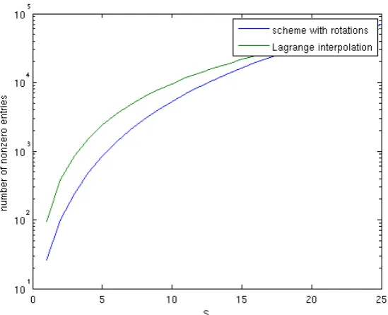
• The interpolation matrices are sparse, which is disadvantageous for computer implementa-tions. For an equivalent number of nonzero entries, it is preferable to have a small, dense matrix, rather than a large, sparse one.

The aim of this research is to examine an alternative scheme with a much lower sample rate for the aggregation of far field radiation patterns. In this scheme, the far field radiation pattern is rep-resented by its coefficients with respect to the spherical harmonics, which are the analog on the surface of the unit sphere of the Fourier basis functions in 1D. The current research is inspired by the work of Eibert [13] who stored the far field radiation patterns at the finest (with the smallest clusters) level in spherical harmonics, rather thank-space samples. His motivation is to reduce the memory requirements of the MLFMA. In the algorithm presented in this report, the far field radiation patterns are also represented by spherical harmonics at the higher (with larger clusters) levels. The effect of a shift on the spherical harmonics coefficients of a far field radiation pat-tern is computed directly, and thek-space samples are only reconstructed for the application of the transfer functiongc1c2(ˆk). An arbitrary shift can be decomposed into a rotation, a shift along

the z-axis, and the inverse rotation, which results in a computational complexity ofO(K32), with

Kthe sample rate, in this case the number of spherical harmonics coefficients. This decompo-sition is also used in the different context of the low-frequency multilevel fast multipole algo-rithm [34]. Following [18], we will call this the RCR-decomposition, where R stands for rotation and C stands for coaxial translation. A further innovation is use of the real spherical harmon-ics, which is advantageous for the efficiency of the implementation. To our knowledge, the real spherical harmonics have not been used before in the aggregation phase of the MLFMA. The motivation for the present strategy is that sample rate is reduced by a factor of up to eight compared to the standard method. It is expected that this will result in lower CPU times. The disadvantage of the new scheme is that its computational complexityO(K32)is higher than for

(9)

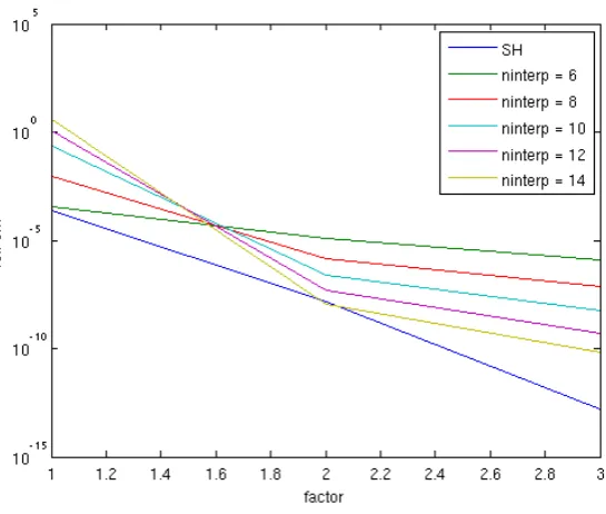
ef-ficient. At the higher levels, where the clusters increase in size, it is better to switch to Lagrange interpolation for its smaller computational complexity and better parallellization capabilities. The new scheme is a global interpolator and a bandlimited function is reproduced exactly if suf-ficient spherical harmonics are used. Far field radiation patterns are not exactly bandlimited, and the interpolation error decays exponentially with the number of spherical harmonics, rather than linearly with the number ofk-space samples in Lagrange interpolation. If a low sample rate with few spherical harmonics is used, then the interpolation error is of comparable size to Lagrange interpolators.

To our knowledge, this is the study where the use of spherical harmonics expansions in the ag-gregation phase of the MLFMA as a means of reducing the sample rate is worked out in detail, including an examination of the error due to the shifts and CPU time measurements where we compare the scheme to Lagrange interpolation. Other schemes in the literature for reducing the sample rate in the aggregation phase of the MLFMA are based on trigonometric polynomial ex-pansions and the fast Fourier transform [31], [6], [22], [23]. These schemes also result in a re-duction of the sample rate by a factor of eight, but this rere-duction is only achieved for large clus-ters, where we intend to switch to Lagrange interpolation with parallellization over the direc-tions.

The structure of this report is as follows. In Chapters 2-4 we give a summary of scattering prob-lems, the weak formulation and the numerical discretization. In Chapter 5 we describe the fast multipole method as a starting point for our discussion of the standard MLFMA in Chapter 6. In Chapter 7 we describe the use of spherical harmonics coefficients as a representation of the far field radiation patterns at the finest level in the MLFMA. This technique was introduced as a means of saving memory in [13] and the algorithm presented in this report can be seen in some ways as an extension of this technique to the higher levels. In Chapter 8 we discuss the use of spherical harmonics expansions at the higher levels, including the RCR decomposition. In Chap-ter 9 we provide CPU time measurements and memory estimates. In ChapChap-ter 10 the possibilities for extensions of the algorithm to reduce the computational complexity are discussed. Finally, we conclude with a discussion of our results in Chapter 11.

2

Scattering problems

In this chapter scattering problems are described. The visibility of an aircraft (or another object like a bird) on a radar system is measured by its radar-cross section, which is computed for a given time-harmonic incident electric field

(10)

representing ground-based and aircraft-mounted radar systems. Radar-cross section computa-tions are based on the electric field integral equation (EFIE), which is derived in [7]. Define the operator

L(X) =ik

ˆ

S

X(r0)φ(r,r0)− 1

k2(∇

0_·_X₍_r0₎₎_∇0_φ₍_r_,_r0₎_d_r0

t

, (4)

with(·)_tthe tangential part,Sthe scatterer,k = ω/cthe spatial frequency,ωthe angular fre-quency,cthe speed of light,∇0 _{the gradient with respect to the integration variable}_r0_,_r _{the field} variable, andφthe Green’s function

φ(r,r0) = e

−ik|r−r0|

|r−r0_| . (5)

The scattererSis the boundary∂Ωof the regionΩsurrounding the scatterer. Let the impedance in free space be given by

η=

r

µ0

0

, (6)

withε0andµ0the free-space dielectric constant and permittivity, respectively. The scatterer is modeled as a perfect electric conductor, with a fictitious surface-currentJsthat completely can-cels the incident electric field. The EFIE is given by

ηL(Js) = 4πEtinc. (7)

The operatorLcan be interpreted as the electric field generated by a current distributionJs mul-tiplied by the constant−4π

η . The scattering problem consists of computing the currentJsgiven an incident electric fieldEinc. The radar-cross section can be computed usingJs. The operator

(11)

3

Weak formulation

In this chapter the weak formulation of the EFIE is given. Define the following two bilinear op-erators

L₁(X,Y) = ˆ

S

ˆ

S

φ(r,r0)X(r0)·Y(r)dr0dr,

L₂(X,Y) = ˆ

S

ˆ

S

(∇0·X(r0))φ(r,r0)(∇ ·Y(r))dr0dr.

LetW be a test-vector field that is tangential to the surface, and that is an element ofH−12(div),

the space of vector functionsf for which

ˆ

S

ˆ

S

f(r)·f(r0₎

R dr

0_d_r ₊

ˆ

S

ˆ

S

∇ ·f(r)∇0_·_f₍_r0₎

R dr

0_d_r

is finite. This function space follows from the trace theorem in functional analysis and the as-sumption that the electric field and its divergence have finite energy, in other words, that they are locally square integrable. Details can be found in [21]. The tangential trial-vector fieldJsis also an element ofH−12(div). The weak formulation is then given by

ˆ

S

4πW ·E_tincdr = ikη(L1(W,Js)−

1

k2L2(W,Js)). (8) Again, the details can be found in [21].

4

Discretisation

The RWG basis functions from Rao, Wilton and Glisson [29] are used on a piecewise linear ap-proximation of the surface with triangular elements. These basis functions are defined for each edge, that is not on the boundary of the surface (in the case that it is not closed)

fj(r) =







± l

A±(r−r

±₎ _r_∈_T±

0 elsewhere

, (9)

withT±the two triangles incident to the edge,lthe length of the edge,A±the areas of the tri-angles andr±the corner points opposite the edge. The basis functions are illustrated in Figure 1. The currentJsis approximated as a linear combination ofN basis functions

Js=

N

X

j=1

(12)

Fig. 1 RWG basis function

For the test functions the same basis elements are used. The following linear system is then found

ˆ

S

fi·4πEtincdr = N

X

j=1

ηLijJj, , i= 1, . . . , N, (11)

with

L_ij =L(fi,fj), (12)

and

L= ik(L1+

1

k2L2). (13)

5

Fast multipole method

In this chapter the fast multipole method is described. The linear system (11) is solved using a Krylov iterative method, in which the system matrix is required only for matrix-vector products. It can be seen that the system matrix is full, and that the complexity of the matrix-vector products is thereforeO(N2). For radar-cross section computations with a realistic size the system matrix is too large even to be stored in memory. The fast multipole method (FMM) improves the CPU and memory requirements toO(N√N).

[image:12.595.217.436.110.307.2]

(13)

of the fast multipole method with the goal of clarifying the physics behind it. The entries of the system matrix are given by

L_ij = ˆ

S fi(r)·

−4π

η [E(fj)](r)dr, (14)

which express the interaction of the electric fieldE(fj)induced by the source currentfj with the basis functionfi. The basis function related to the test function is interpreted as the sensitivity at

r of the surface to the electric field. Note that the basis functions are seen as scatterers in their own right. The fast multipole method is based on the idea that the electric field outside a current distribution can be reconstructed from the electromagnetic far field [11]. Recall that in scattering problems we seek solutions to the Helmholtz equation

∇2E(r) +k2E(r) =0. (15)

We will solve the Helmholtz equation in the exterior ofB(0, d), the sphere centered in0, with radiusdchosen so that the source currentfjis contained inside. In scattering problems it is con-ventional to apply the Sommerfeld radiation condition, see [24] for a discussion. If this condition is applied, then the electric field has the following multipole expansion outside the sphere

E(rˆr) =

∞

X

p=0 p

X

q=−p

Epqh(2)_p (kr)Y_pq(ˆr), (16)

withˆrthe unit vector in the direction ofr,r = |r|,Epqthe spherical harmonics coefficients of the electric field,h(2)p the spherical Hankel function of the second kind, andYpq(ˆr)the spherical harmonics, given in spherical coordinates by

Y_pq(θ, φ) := (−1)q

(p−q)! (p+q)!

2p+ 1 4π

1/2

P_pq(cos(θ))eiqφ,

withpthe degree,qthe order, andPpqthe associated Legendre polynomial of degreepand order

(14)

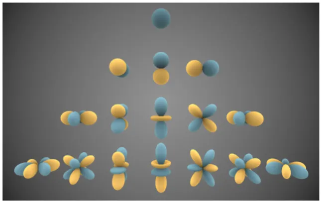
Fig. 2 real spherical harmonics(73). They are ordered by degree from top to bottom and by order from left to right. Blue regions indicate where the functions are positive. The

dis-tance from the origin indicates the magnitude. Figure from Inigo.quilez. 14 May 2014 viahttp://commons.wikimedia.org/wiki/File:Spherical Harmonics.png, Creative Commons Attribution-Share Alike 3.0 Unported

the Helmholtz equation due to a bounded current distribution have a limit in the far fieldr → ∞, given by [5]

E(rˆr) = (I−rˆrˆ)

−ike−ikr

4πr

ˆ

S

fj(r0)eikr 0_·ˆ_r

dr0, r → ∞, (17)

with(I−rˆrˆ)the projection operator

v 7→v−(ˆr ·v)ˆr. (18)

The angular dependence(I−rˆrˆ)´_Sfj(r0)eikr 0_·ˆ_r

dr0is called the far field radiation pattern. They are also sometimes called outgoing waves in the literature, because the terms in the multipole expansionEpqh(2)p (kr)Ypq(ˆr)are spherical waves propagating outward. The spherical Hankel functions of the second kind have the following limit behavior

h(2)_p (kr)→ (i)

p+1_e−ikr

kr , (19)

asr → ∞. By taking the limit asr → ∞in (16), and equating it to (17), we can reconstruct the spherical harmonics coefficients of the electric field

Epq = −k

2

4π(i)p

ˆ

ˆ S

(I−kˆkˆ)

ˆ

S

[image:14.595.164.488.111.319.2]

(15)

withSˆthe unit sphere (not to be confused with the complement of the domain in which we are solving the Helmholtz equation),(·)∗the complex conjugate, and where we have used the nota-tionkˆinstead ofˆr. Thekˆare called directions in [8]. Following [13], integrals over the surface of the unit sphere are calledk-space integrals. The electric field is then given by

E(rˆr) =

∞ X p=0 p X q=−p

h(2)_p (kr)Y_pq(ˆr) −k

2

4π(i)p

ˆ

ˆ S

(I−kˆkˆ)

ˆ

S

fj(r0)eikr0·kˆdr0Y_pq∗(ˆk)dˆk. (21)

We absorb the summation over the order into thek-space integral overSˆ

E(rˆr) =

∞

X

p=0

h(2)_p (kr) −k

2

4π(i)p

ˆ

ˆ S

(I−kˆkˆ)

ˆ

S

fj(r0)eikr0·ˆkdr0

p

X

q=−p

Y_pq(ˆr)Y_pq∗(ˆk)dkˆ. (22)

Spherical harmonics of degreepare homogeneous polynomials of degreep. The set of homo-geneous polynomials of degreepis invariant under a rotation. Therefore, spherical harmonics in the spherical coordinate system where the North pole matches the vectorˆrcan be expressed as a linear combination of spherical harmonics in the Cartesian coordinate system, where the North pole matches the vectorez. In fact, we have for the spherical harmonic with order zero in the rotated coordinate system that

2p+ 1

4π Pp(ˆk·ˆr) =

p

X

q=−p

Y_pq(ˆp)Y_pq∗(ˆk), (23)

withPpthe Legendre polynomial of degreep. See [3] for details about the special functions. We then find for the electric field

E(rˆr) =

∞

X

p=0

h(2)_p (kr)−k

2₍₂_p_{+ 1)}

(4π)2_(i)p

ˆ

ˆ S

(I−kˆkˆ)

ˆ

S

fj(r0)eikr 0_·_k_ˆ

dr0Pp(ˆk·ˆr)dkˆ. (24)

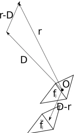
It is seen that we have reconstructed the electric field for all points withr > dbased on the far field. Unfortunately, the current situation is not yet satisfactory. Sincer0andˆrare present in the same integral, we still end up needing to calculate the interactions separately for all pairs of basis functions, and we know from before that this results in a system matrix that does not fit into the computer memory. Fortunately, this problem is easily solved. We apply the following decomposition

r =D+r−D, (25)

whereD is some vector. Instead of computing[E(fj)](r)for many values ofr, we can also compute[E( ˜fj)](D)for a fixedD, but with displaced source currents

˜

(16)

r

D

r-D

D-r

O

f

j

f

j

~

Fig. 3 original and displaced current distribution

The original and displaced current distribution are illustrated in Figure 3. The far field of this displaced source current is

E(rˆr) = (I−rˆrˆ)

−ike−ikr

4πr

ˆ

˜ S

˜

fj(r0)eikr 0_·ˆ_r

dr0, (27)

withS˜the displaced scatterer. We apply a change of variablesr0 →r0+r−D and find that the far field is given by

E(rˆr) = (I−rˆrˆ)−ike −ikr

4πr

ˆ

S

fj(r0)eik(r0−(r−D))·ˆrdr0. (28) We can take out the new exponential factor and compute the electric field using (24), where, as mentioned, we substituterˆr=DDˆ and the displaced source current to calculate the electric field atrˆrdue to the original source current

E(rˆr) =

∞

X

p=0

h(2)_p (kD)−k

2₍₂_p_{+ 1)}

(4π)2_(i)p

ˆ

ˆ S

eik(−(r−D))·kˆ(I−kˆkˆ)

ˆ

S

fj(r0)eikr 0_·_k_ˆ

[image:16.595.262.390.111.339.2]

(17)

an infinite sum for every basis function that is related to a test function. Therefore we truncate the multipole expansion atp=P and interchange the integration and summation to obtain

E(rˆr)≈

ˆ

ˆ S

eik(−(r−D))·ˆk





P

X

p=0

h(2)_p (kr)−k

2₍₂_p_{+ 1)}

(4π)2_(i)p Pp(ˆk·Dˆ)



(I−kˆkˆ)

ˆ

S

fj(r0)eikr 0_·_kˆ

dr0dkˆ.

(30) We now have an expression that is suitable for a numerical method, becauser andr0appear in different integrals. This means that the interactions between basis functions can be computed in clusters of basis functions. Suppose that we have two clustersGmandGm0 and that we want to compute the interactions between the basis functions inGm0 with the electric field due to the basis functions inGm

X

j∈Gm

L_ijJj =

ˆ

S fi(r)·

−4π η [E(

X

j∈Gm

Jjfj)](r)dr, i∈Gm0, (31)

withJj the surface current expansion coefficients. We then compute these interactions in three steps:

far field radiation pattern due to the current sourceP

j∈GmJjfj

ˆ

S

X

j∈Gm

Jjfj(r0)eikr 0_·ˆ_k

dr0.

transfer to a location in the center of clusterGm, given by position vectorD, by multiplication with the transfer function





P

X

p=0

h(2)_p (kr)−k

2₍₂_p_{+ 1)}

(4π)2_(i)p Pp(ˆk·Dˆ)



.

receiving patterns which are given by

ˆ

S

fi(r0)e−ikr0·kˆdr0.

The term receiving pattern is from [8].

The product of the transfer function and the far field radiation pattern is called an incoming wave in the literature. This term is related to a somewhat different derivation of the fast multipole method using a multipole expansion of a different type. We will not discuss this subject, but de-tails can be found in [12] and [8].

(18)

There are some caveats. The transfer function (the sum inside thek-space integral in (30)) is actually divergent if we letp → ∞, since the interchange of the summation and the integral is not a mathematically valid operation. This can cause numerical problems in some situations, see Section 6.3.

We also need to carefully examine on what domain expression (30) is valid. We had earlier as-sumed thatfj is contained insideB(0, d). Suppose that we want to evaluate the electric field in a unit sphereB(D, d), centered inD. This is what we are doing in the example with clusterGm0 above. Then the displaced currents are contained insideB(0,2d)and the expression for the elec-tric field is valid forD >2d. This condition must not be violated in the FMM.

We can give the following physical interpretation of the incoming waves. The incoming waves are the coefficients in an (approximate) plane wave expansion of the electric field in the sphere

B(D, d)due the current source in the sphereB(0, d). Note that this does not explain the name incoming waves.

As mentioned, an essential feature of the FMM is that interactions between basis functions are computed in clusters. We previously described how to compute the interactions between basis functions in two clustersP

j∈GmLijJj. We will now describe the FMM where interactions are

computed between all the basis functionsPN

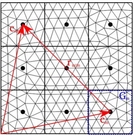
j=1LijJj. For this, a cubic lattice is superimposed on the mesh. The analogous 2D case where a square lattice is superimposed on the mesh is il-lustrated in Figure 4. Each basis function is assigned to the cube containing the mid-point of its edge. We use the term cluster to denote the set of basis functions in a nonempty cube. Define

Gm, the set of basis functions in clusterm, andcm, the center of the cube corresponding to clus-term.

(19)

c

m'

c

m

r

m'm

G

m

Fig. 4 interaction between two clusters in the FMM on a part of a plate mesh in the 2D case.

The circles are cluster centers and the thick line segments are the edges of clusters. The thin line segments are edges corresponding to basis functions. The dashed blue line segments illustrate what basis functions are contained in clusterGm.

FMM.

With these preliminaries out of the way, we can describe the FMM approximation to the matrix-vector products

J_ioutput =

N

X

j=1

LijJ_jinput≈ik

ˆ

ˆ S

ˆ

S

fie−ik ˆ

k·(r0₋_c

m0)_d_r0

| {z }

receiving pattern

·

X

m /∈Gadj

m0

α(kkˆ,rm0_m)

| {z }

transfer

X

j∈Gm

(I−kˆkˆ)

ˆ

S

fjeik ˆ

k·(r−cm)_d_r

| {z }

far field radiation pattern

J_jinputdkˆ

+ X

m∈Gadj

m0 X

j∈Gm

LijJ_jinput,

withm0the cluster containing basis functioni,J_ioutputthei-th component of the output vector in the Krylov iteration, corresponding to basis functioni,J_jinputthej-th component of the input vector at iterationr, corresponding to basis functionj, and

α(kkˆ,rm0_m) := k

4π

P

X

p=0

(−i)p+1(2p+ 1)h(2)_p (k|rm0_m|)P_p(ˆk·ˆr_m0_m),

[image:19.595.219.434.110.327.2]

(20)

Fig. 5 transfer phase in the FMM and the MLFMA. This illustration is also used in the chapter about the MLFMA. Not all clusters are shown. In the FMM, the dark grey cluster also

interacts with clusters that are not shown (that are farther away). In the MLFMA, the ar-rows indicate all the interaction for this cluster. Interactions between basis functions in clusters that are farther away are computed at a coarser level. The light grey indicates

[image:20.595.218.433.267.481.2]

(21)

withh(2)p the spherical Hankel function of the second kind of orderp,P the number of multi-poles, andPpthe Legendre polynomial of degreep. The variables are illustrated in Figure 4. The far field radiation patterns, transfer function and receiving patterns are reused in all matrix-vector products and are precomputed in the initialization phase of the FMM. Thek-space integral over

ˆ

Sis evaluated numerically during the solution phase of the algorithm. More details on numerical quadrature of this integral is given in Section 6.3.

5.1 Derivation

The derivation in this section is gieven in [8]. Let the test and current basis functionsfiandfj be contained in clusters withGm0 andG_m with cluster centersc_m0 andc_mrespectively. Suppose that we are trying to find the electric field atr0, in the domain offi, due to a current atr, in the domain offj. We apply the following decomposition

r0−r =r0−cm0 +c_m0−c_m+c_m−r =:d_m0 +r_m0_m−d_m. (32) Define

d :=dm0−d_m,

D :=rm0_m,

and assume that|d|<|D|. The addition theorem (see [8]) states

e−ik|D+d|

|D+d| =−ik ∞

X

p=0

(−1)p(2p+ 1)jp(kd)hp(2)(kD)Pp( ˆd·Dˆ), (33)

withd = |d|,D = |D|, andjpthe spherical Bessel function of the first kind of orderp. See [3] for details about the spherical Bessel function of the second kind. The following plane-wave expansion can now be applied [8]

4π(−i)pjp(kd)Pp( ˆd·Dˆ) =

ˆ

ˆ S

e−ikˆk·dPp(ˆk·Dˆ)dkˆ, (34)

whereSˆis the unit sphere. We now truncate the expansion (33), apply the plane-wave expan-sion, and interchange the integration and summation to obtain the following approximation to the Green’s function

e−ik|D+d|

|D+d| ≈

ˆ

ˆ S

(22)

with the transfer function

α(kkˆ,D) := k 4π

P

X

p=0

(−i)p+1(2p+ 1)h(2)_p (kD)Pp(ˆk·Dˆ), (36)

andP the number of multipole terms that we keep. Substituting the approximation to the Green’s function into the weak formulation we find

L_ij ≈ik

ˆ

ˆ S

ˆ

S

fie−ik ˆ

k·(r0−cm0)_d_r0

α(kkˆ,rm0_m)(_I−kˆkˆ)

ˆ

S

fjeik ˆ

k·(r−cm)_d_r

dkˆ. (37) In the literature this factorization is called a diagonalization of the transfer operator. This inter-pretation makes more sense in the context of the derivation of FMM in 2D in [8], where two sep-arate multipole expansions are applied and a convolution theorem is applied.

6

Multilevel fast multipole algorithm

6.1 Description of the algorithm

(23)

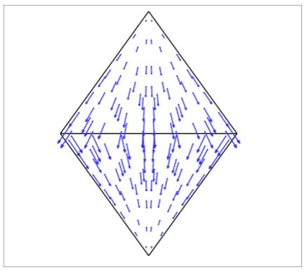
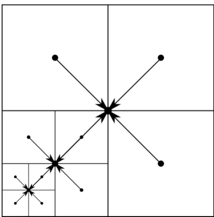
Fig. 6 aggregation in the MLFMA in 2D. The line segments indicate the edges of the boxes. In 3D these become cubes. The thick line segments indicate boxes at coarser levels and

the thin line segments indicate boxes in finer levels. Not all the sub-boxes are shown. The circles indicate box centers. The arrows indicate the shifts in the aggregation. The circle in the center of the figure represents the box center of a single box at the finest

level.

levelsl = 1, . . . , lmax, each cube is recursively subdivided into eight child cubes and only the

nonempty ones are retained. At the finest levellmax, the nonempty cubes contain about10

ba-sis functions. Note that, inconba-sistently with this indexing, the coarser levels were described as higher levels in the introduction to this report. In Figure 6 the octree structure is illustrated in the 2D case. DefineN_gl, the number of clusters (nonempty cubes) at levell. The subscriptgrefers to group, another term that is used for the clusters in the literature. We use the following indices for the clusters at levell

m= 1, . . . , N_gl.

Also, definec_ml , the cube center corresponding to clustermat levell. DefineGl_mforl < lmax,

the set of child clusters of clustermat levell. Furthermore, defineGlmax_m , the set of basis func-tions in clustermat the finest levellmax. In the MLFMA, interactions between basis functions

[image:23.595.218.432.109.326.2]

(24)

integration points used in thek-space integral at levell,kˆ_il, the integration points, andωl_i, the quadrature weights. Recall that the integration points are also the directions used in the aggrega-tion phase in the MLFMA.

A key step in the MLFMA is the use of interpolation. In the interaction between two clusters, we apply a transfer function to the far field radiation patterns. The motivation for interpolation is that the far field radiation pattern of a large cluster has a large spectral content. It therefore needs to be sampled at a large number directions. It is expensive to compute thesek-space sam-ples directly, since this involves integration over the surface of the scatterer. Now a large cluster is composed of a number of child clusters. These are smaller and the spectral content of their far field radiation patterns is also smaller. Their far field radiation patterns are therefore sampled at a smaller number of directions. We use the key step of interpolation to sample them at the larger number of directions of the parent cluster. Thek-space samples of the parent cluster are then computed by summation over the interpolatedk-space samples of the child clusters at each di-rection required for the parent cluster. This idea can also be applied to the child clusters and their child clusters and so on. This recursive process is called aggregation.

We did just neglect one additional step. The spectral content of the far field radiation pattern depends on the origin of the coordinate system with respect to which it is defined. The spectral content is smallest if the origin is at the center of a cluster. Therefore we ensure that the far field radiation patterns are always defined with respect to the cluster centers by applying shifts when aggregating from a finer level to a coarser level. These shifts are illustrated in Figure 6.

We will now describe the MLFMA in detail. It is divided into five stages.

summation over thek-space samples of the individual basis functions in each cluster at the finest level, at each direction

v_m,lmax(o) (ˆk_ilmax) := X

j∈Glmax

m

(I−kˆ_ilmaxkˆ_ilmax)

ˆ

S

fjeik ˆ

klmax

i ·(r−c lmax

m )_d_r_Jinput

j ,

form = 1, . . . , N_glmax,i= 1, . . . , Klmax. The integral overSis precomputed for each value ofkˆ_ilmax. The superscript(o)refers to outgoing waves.

aggregation where the far field radiation patterns at the levelsl=lmax−1, . . . ,2are recursively

aggregated from fine to coarser levels

v_m,l(o)(ˆk_jl) := X

mc∈Glm

eikˆkjl·(c l+1

mc−clm)_v_˜(o)

mc,l+1(ˆk

l j),

form = 1, . . . , N_gl, the directions at the coarser levelj = 1, . . . , Kl, withv˜ (o) mc,l+1(ˆk)

the interpolated far field radiation pattern based on thek-space samples at the finer level

v_m(o)

c,l+1(ˆk

l+1

(25)

samples at the coarser level. This step is illustrated in Figure 6. We used the subscriptcto indicate that an index refers to the child clusters.

transfer of the far field radiation patterns to the cube centers

v_m(i),12_,l(ˆk

l i) :=

X

m1_∈Gint,l m2

ωl_iα(kkˆ_il,c_ml 2 −c_ml 1)v

(o) m1_,l(ˆk

l i),

form2 = 1, . . . , N_gl,l = lmax, . . . ,2. The multipole expansionα(kkˆil,clm2 −c_ml 1)is

precomputed during the initialization phase. We used the superscript(i),1to indicate that these are incomplete incoming waves. The incoming waves (coefficients of the approxi-mate plane wave expansion of the electric field) computed in this step are only due to the source currents in clusters that interact at this level, instead of all the clusters. Note that the quadrature weights are applied at this step.

disaggregation where the incoming waves at the levelsl= 3, . . . , lmax1are disaggregated from

the coarser to the finer level

v_m,l(i),2(ˆk_jl) :=e−ikˆkjl·(c l−1

mp−cml)_v_˜(i),2

mp,l−1(ˆk

l j) +v

(i),1 m,l (ˆk

l j), formp = 1, . . . , Ngl−1, for allm∈Gl−1mp,j = 1, . . . , Kl, withv˜

(i),2

mp,l−1(ˆk)the interpolated

incoming waves based on the sample valuesv_m(i),2_p_,l−1(ˆk_il−1)at the directions correspond-ing to the coarser leveli = 1, . . . , Kl−1. The interpolated incoming waves are sampled at the directions corresponding to the finer levels. Since there are fewer of these, we are undersampling the incoming waves. Note that in the disaggregation phase, the spectral content of the incoming waves is not expected to depend on the level. The reason for this is that the incoming waves represent the plane wave coefficients of the electric field (by ap-proximation) due to current sources clusters that interact at this level or coarser levels. The electric field due to these has a larger spectral content than the electric field due to source currents in cluster that interact at finer levels or due to source currents in the buffer zone. The interpolations in this step are called anterpolations in the literature. They are the trans-pose of the interpolations in the aggregation. We use the subscriptpto indicate the parent clusters.

testing where the new current coefficient vector is computed

J_joutput:= ik

Klmax

X

i=1

(I−kˆilmaxkˆ lmax i )

ˆ

S

fje−ik ˆ

klmax

i ·(r−cmmax)_d_r ·_v(i),2

m,lmax(ˆk lmax i ),

forj = 1, . . . , N, withmthe cluster that basis functionjis located in. The integral overS

is precomputed for each value ofkˆ_ilmax.

(26)

The term far field radiation patterns is used to describe different things in this report. The first possibility refers to the far field radiation patterns computed recursively above. It is also used to describe

X

j∈Gbm,l

ˆ

S

fjeik ˆ

kl

i·(r−cml )_d_r_, ₍₃₈₎

withGbm,lthe set of basis functions in clustermat levell. The far field radiation patternsv_m,l(o) computed using the MLFMA are approximations of the above integral.

6.2 Lagrange interpolation in the MLFMA

Interpolation is an essential step in the MLFMA because it is too expensive to directly sam-ple the far field radiation patterns directly at the coarser levels, corresponding to large clusters, where they have a large spectral content. Recall that we apply interpolation during the aggrega-tion phase of the MLFMA, where we have thek-space samples of the far field radiation pattern at some level, and we use interpolation to find thek-space samples at the larger number of direc-tions of the coarser level.

The standard interpolation method for the MLFMA in the literature is Lagrange interpolation. In this section we describe Lagrange interpolation. The directions used in the aggregation process match the integration points in thek-space integrals in the MLFMA. The continuous versions of thek-space integrals in the MLFMA are not given in this report, but they are similar to (32). The use of the integration points as directions in the aggregation is actually oversampling of the far field radiation patterns, but it is necessary in order to obtain a sufficiently small interpolation error.

We will now describe the integration points. LetLbe some positive number. The integration points are the Gauss-Legendre quadrature points(θj, φi),j= 1, . . . , L,i= 1, . . . ,2L. In Gauss-Legendre quadrature, there are2Lequally-spaced integration points in theφdirection, and the points in theθdirection are theLzeros ofPL, the Legendre polynomial of degreeL.

In our implementation, we use a2p×2pstencil for the interpolation, wherepis an interpolation parameter. In our implementation, we usep= 3, resulting in an interpolation error that is smaller than= 0.001in our tests. The formula for Lagrange interpolation in the scalar case is

˜

f(θ, φ) =

s+p

X

i=s+1−p

ωi(φ) t+p

X

j=t+1−p

vj(θ)f(θj, φi), (39)

withf˜(θ, φ)the interpolated function andf(θj, φi)the sample values at the interpolation points

(θj, φi). We have that(t, s)depends on the target point(θ, φ). The interpolators are given by

ωi(φ) =

s+p

Y

k=s+1−p,k6=i

φ−φk

φi−φk

(27)

and

vj(θ) =

t+p

Y

l=t+1−p,l6=j

θ−θl

θj −θl

. (41)

We actually use a two-step process for the Lagrange interpolation, in order to reduce CPU times. In the first step we determine interpolationsf˜1(φ, θi), separately for all values ofθi correspond-ing to sample points at the previous level, and we evaluate the interpolations at all theφ = φj corresponding to target points at the new level. In the second step we determine interpolations

˜

f2(φj, θ), separately for all values ofφj corresponding to target points at the new level, and we evaluate the interpolations at the target pointsθ=θlcorresponding to the new level.

6.3 Parameters and error sources in the MLFMA

There are two important parameters in the MLFMA that we will discuss together with their asso-ciated errors in this chapter:

• The choice of directionskˆl_jand the integration error,

• The number of multipole termsPlin the transfer functionα(kkˆil,clm2_l −c l

m1_l)and the truncation error.

We will also discuss the interpolation error. 6.3.1 Choice of directions

Recall that the directionskˆl_j at levellin the aggregation in the MLFMA match the integration points at that level in thek-space integral. The reasons for this are that accurate Lagrange inter-polation requires oversampling of the far field patterns and that reconstruction of large number ofk-space samples from a smaller number introduces a new CPU cost. It is awkward to write down thisk-space for the MLFMA and we have not done so in this report. The integration points are determined by the requirement that the numerical integrationk-space integral is accurate. In order to avoid a mess of notation we will consider the choice of integration points in thek-space integral in the FMM

ˆ

ˆ S

ˆ

S

fie−ik ˆ

k·(r0₋_c

m0)_d_r0

| {z }

receiving pattern

· X

m /∈Gadj

m0

α(kkˆ,rm0_m)

| {z }

transfer

X

j∈Gm

(I−kˆkˆ)

ˆ

S

fjeik ˆ

k·(r−cm)_d_r

| {z }

far field radiation pattern

J_jinputdkˆ.

(28)

integration points isK = 2L2. The error due to numerical integration of thek-space integral is negligible if sufficient integration points are used [25], namelyL = P + 1.2 The key idea here is that, due to the orthogonality of the spherical harmonics used in the underlying analysis, only polynomial terms in the integrand in thek-space integral up to degree2P have a nonzero contribution to the integral, and these can be numerically integrated exactly forL = P + 1. The integration error is then due to polynomial terms with degree2P + 1and higher, that ana-lytically integrate to zero but not numerically. In practice, the integration error is much smaller than the error due to the truncation of the multipole expansion and the interpolation error. The extension to the MLFMA is immediate. We then find that the number of directions is given by

Kl= 2(Pl+ 1)2, withPlthe number of multipole terms. 6.3.2 Number of multipole terms

Finally, we will consider the number of multipole termsPlin the transfer functionα(kkˆil,cml 2 l

−

c_ml 1

l). In the literature, the relative error in either (33) or (35) of the FMM due to the truncation

of the multipole expansion is analyzed. This is also called the truncation error in the literature. The results can be immediately extended to the MLFMA. We make the following remarks on these analyses:

• The asymptotic analyses of the relative error in (33) in [8] and [32] are parameter-dependent. They rely on assumptions such as D_d → ∞,kd→ ∞and other approximations, that need to be validated empirically for our problem parameters. We have found in fact, that the analyses in [8] and [32] are invalid for our parameters.

• In computer implementations, the relative error in (35) is not controllable to arbitrary pre-cision by using a high enoughP, because the transfer function (36) is a divergent series, and we cannot accurately subtract very large numbers in finite precision arithmetic [20]. This is called the low-frequency breakdown. This divergence is a result of the fact that the interchange of the series and integral in the derivation of (35) is not mathematically valid if the series is not truncated. In levels where the cube diameterdlis small compared to the wavelength, this severely constrains the obtainable accuracy. In fact, the relative error in (35) is not controllable to accuracy = 0.001for certaindandDin the levels with

dl< λ.

In [8] the so-called excess bandwidth formula is derived using asymptotic analysis. This is an estimate of the number of multipole terms required to approximate the Green’s function (33) withd0digits of accuracy

Pl =kdl+ 1.8d2/30 (kdl)1/3, (43) 2

(29)

l Pl Kl

11 6 128

10 8 200

9 12 392

8 19 882

7 31 2178

6 54 6272

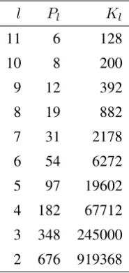
[image:29.595.115.208.113.309.2]

5 97 19602 4 182 67712 3 348 245000 2 676 919368

Table 1 Characteristics of the MLFMA for a realistic aircraft at 10GHz

withdlthe cube diameter at levell. In this report, we used0 = 3, which is satisfactory for radar-cross section computations. Our tests indicate that this formula underestimates the required num-ber of multipoles fordl < λ. However, integral tests of the MLFMA performed at the National Aerospace Laboratory indicate that this does not result in an overall relative error that is larger than= 0.001. In Table 1 the number of multipoles and directions at the different levels is given for a realistic simulation. The cube diameter at the finest level isdc = 0.25λ. The diameterdlof the cubes at levellis given by

dl= 2ldc.

6.3.3 Interpolation error

We define the interpolation error for a clustermlat levellas

l= max

ˆ

kl i

|v_m(o)

l,l(ˆk

l i)−

P

j∈Gb_ml,l

´

Sfje ikˆkl

i·(r−clml)_d_r_|

|P

j∈Gb

ml

´

Sfje ikkˆl

i·(r−cmll )_d_r_|

,

withGbm,ll the set of basis functions in clustermlat levell. The interpolation error is of the same

(30)

7

Spherical harmonics expansion of the far eld radiation patterns of

the individual basis functions at the nest level

In this chapter the scheme from [13] is described, which reduces the sample rate of the far field radiation patterns of the individual basis functions at the finest level by a factor of eight. The mo-tivation is to reduce the memory requirements of the MLFMA. These are dominated by the costs of storing the far field radiation patterns of the individual basis functions at the finest level. These need to be stored for all the individual basis functions, whereas the interpolation matrices at the higher levels can be applied to many different clusters. Recall that in the standard MLFMA we store the far field radiation pattern at the finest level ink-space samplesv_j,m(o)

lmax+1, at the

direc-tionskˆ_ilmax. This is called thek-space representation in [13]. It is possible to use an interpolation strategy to reproduce the the far field radiation pattern based on a smaller number of underlying functions. The interpolants are given by the spherical harmonics

Y_pq(θ, φ) := (−1)q

(p−q)! (p+q)!

2p+ 1 4π

1/2

P_pq(cos(θ))eiqφ, (44)

withpthe degree,qthe order, andPpqthe associated Legendre polynomial of degreepand order

q[3]. The spherical harmonics are the analog on the unit sphere of the Fourier basis functions in 1D. The spherical harmonics are an efficient representation of functions where the spectral content is concentrated in the lower frequencies, as is the case for the far field radiation patterns. A key property of the spherical harmonics is that they are an orthonormal basis for functions on the unit sphere in theL2-inner product. The spherical harmonics expansion of a scalar functionf

on the surface of the unit sphere is given by

f(ˆk) =

S

X

p=0 p

X

q=−p

fpqYpq(ˆk), (45)

withSthe degree of the spherical harmonics expansion and spherical harmonics coefficients

fpq =

ˆ

ˆ S

f(ˆk)Y_pq∗(ˆk)dkˆ, (46) with(·)∗the complex conjugate. The central idea in this chapter is to store the spherical harmon-ics coefficientsfpq of the far field radiation patterns of the individual basis functions at the finest level rather than thek-space values, and to reconstruct thek-space values (which are multiplied by the transfer function in the MLFMA) for all the clusters at the finest level during the itera-tions.

(31)

far field radiation patterns have a limited spectral content. Due to this rapid decay the spherical harmonics expansion can be truncated atS = Plmax/2. It is straightforward to show that a spher-ical harmonics expansion of degreeS contains(S + 1)2 terms. This means that the sample rate is(Plmax/2 + 1)2if the spherical harmonics expansion is used. On the other hand, in the standard MLFMA the far field radiation patterns for the individual basis functions are stored at2P_lmax2 di-rections. This suggests that the interpolation strategy reduces the required amount of memory by a factor of about eight. On the other hand, if the spherical harmonics expansion is used to store the far field radiation patterns, all three Cartesian components need to be stored due to the Gibbs phenomenom, whereas for thek-space representation only the tangential components need to be stored [13]. The Gibbs phenomenom is a result of the fact that the unit vectors in the spherical coordinate system are discontinuous at the poles. That said, the spectral content of the Cartesian components of the far field radiation patterns is smaller than that of the tangential components. Therefore it is expected that the reduction in memory is between a factor of five and a factor of eight [13].

As a motivation, we will discuss why so many directions are used in the ordinary MLFMA. Re-call that the fast multipole method is based on thek-space integrals

ik

ˆ

ˆ S

ˆ

S

fie−ikkˆ·(r0−cm0)_d_r0

α(kkˆ,rm0_m)

(I−kˆkˆ)

ˆ

S

fjeikˆk·(r−cm)_d_r

dkˆ. (47)

The far field radiation patterns(I−kˆkˆ)´_Sfjeikˆk·(r−cm)dr

decay rapidly forp > Plmax/2 if they are represented by spherical harmonics. The receiving patterns

´

Sfie

−ik_kˆ·(r0−c_m0)_d_r0 also decay rapidly forp > Plmax/2if they are represented by spherical harmonics. The trans-fer functionsα(kkˆ,rm0_m)decay rapidly forp > P_lmax. The truncation number is two times as large in the transfer function as in the far field radiation pattern, due to the fact that|r_m0_m| >

2d := 2 maxr(r−cm). Heredis one-half the cube diameter, andrm0_mis the distance over which the interactions between the clusters are computed. In the MLFMA we have|r_m0_m| ≈

2d:= 2 maxr(r−cm). It can now be seen that the quadrature rule must be chosen so that poly-nomials of degree2Plmax are integrated exactly. The required number of integration points is then

(32)

using the formula

ˆ

ˆ S

(I−kˆkˆ)

ˆ

S fjeik

ˆ

k·(r−cm)_d_r

Y_pq(ˆk)∗dkˆ. (48)

We only need to be able to determine the spherical harmonics coefficients up to degreePlmax/2. If the far field radiation patterns are stored ink-space samples, then the spherical harmonics co-efficients are not actually reconstructed in the algorithm, but the spherical harmonics up to de-greePlmax/2need to be implicit in the stored far field radiation pattern, for the validity of the truncation error analysis in the literature. We then need to be able to integrate exactly a polyno-mial of degreePlmax. For this, we needPlmax2 /2directions. This is already a considerable reduc-tion of the sample rate. However, the sample rate is only reduced by a factor of four, instead of a factor of eight if the spherical harmonics are used. This also means that the reconstruction of thek-space samples at the integration points of (47) will be more expensive than if spherical har-monics coefficients are stored.

7.1 Detailed description

The summation step of the MLFMA (see Section 6) is modified in the following way:

summation over the spherical harmonics coefficients of the far field radiation pattern of the in-dividual basis functions in each cluster at the finest level

f_rsm := X

j∈Glmax

m

ˆ

ˆ S

v_j,lmax+1(o) (ˆk)Y_rs∗(ˆk)dkˆJ_jinput,

form = 1, . . . , N_glmax,r = 0, . . . , S,s = −r, . . . , r, and withv_j,lmax+1(o) the far field radiation pattern for the individual basis functions

v_j,lmax+1(o) (ˆk) := ˆ

S

fjeik ˆ

k·(r−clmax

m )_d_r_.

Thek-space integral is precomputed in the initialization phase of the algorithm. reconstruction of thek-space samples at the finest levellmax

v_m,lmax(o) (ˆk_ilmax) :=

S

X

r=0 r

X

s=−r

Y_rs(ˆk_ilmax)f_rsm,

form = 1, . . . , N_glmax. If this expansion is implemented naively, then the computational complexity isO(S4). Using a trivial modification this can be accelerated toO(S3), and using the fast spherical harmonic transform it can be accelerated toO(S2logS)[30]. In the actual algorithm we include quadrature weights

q

ωSˆ

(33)

the application of the transfer function are the transpose of the steps taken before the ap-plication of the transfer function. This does not have a physical interpretation. The trivial modification is described in Section 8.6.

The testing step (see Section 6) is also modified:

spherical harmonics expansion of the incoming waves at the finest levellmax

gm_rs:=

Klmax

X

i=1

ω_iSˆv_m,lmax(i),2 (ˆk_ilmax)Y_rs∗(ˆk_ilmax),

form= 1, . . . , N_glmax,r = 0, . . . , S,s=−r, . . . , r. Note that we use sufficient integration points in this numerical integration, becauseKlmax is sufficient to integrate polynomials of degree2Plmax and the incoming wavesv_m,lmax(i),2 decay rapidly forp > Plmax. In the algorithm we actually use quadrature weights

q

ωS_iˆso that the steps taken after the application of the transfer function are the transpose of the steps taken before the application of the transfer function. This does not have a physical interpretation.

testing where the surface current expansion coefficient vector in the new Krylov iteration is computed

J_joutput:= ik

S

X

r=0 r

X

s=−r

(f_rsj,m)∗·gm_rs,

forj = 1, . . . , N, withmthe cluster that basis functionjis located in, and withfrsj,m the spherical harmonics coefficients of far field radiation patterns of the individual basis functions

f_rsj,m := ˆ

ˆ S

v_j,lmax+1(o) (ˆk)Y_rs∗(ˆk)dkˆ,

which are the conjugate transpose of the receiving patterns. Thefrsj,mare precomputed. In the derivation of the testing step the orthogonality of the spherical harmonics is used. We use spherical harmonics expansions of the same degree (up top = Plmax/2) to represent both the far field radiation patterns and the incoming waves, despite the higher spectral content of the incoming waves. We are here following the argument in [13] that the spherical harmonics coefficients of the incoming waves, which decay rapidly forp > Plmax, are multiplied by the spherical harmonics coefficients of the receiving pattern in the final testing step, which decay rapidly forp > Plmax/2.

7.2 Use of symmetry to reduce the sample rate

In [13] it is mentioned that the symmetry of the far fields radiation patterns

(34)

has been used to reduce the storage costs. In [13] the complex spherical harmonics, were used to store the far field radiation patterns. The complex spherical harmonics are the spherical harmon-ics that have been used so far in the report. The effect of the symmetry on the coefficients with respect to the spherical harmonics is

Ref_rsj,m = (−1)r+sRefr,−sj,m∗, (50)

Imf_rsj,m = −(−1)r+sImfr,−sj,m∗. (51)

The symmetry can be used to realize a reduction in memory requirements by reconstructing the spherical harmonics coefficients for negative order based on the spherical harmonics coef-ficients for positive order during the solution phase of the algorithm. The spherical harmonics coefficients for negative order then do not need to be explicitly stored in the computer’s mem-ory, resulting in memory savings. The number of spherical harmonics coefficients that need to be stored is then decreased by a factor of about two. The same trick can of course also be applied to the ordinary MLFMA by storing thek-space samples only on one-half of the unit sphere.

8

Spherical harmonics based aggregation

8.1 Applying shifts to the spherical harmonics expansions

The spherical harmonics representation of the far field radiation pattern can also be used at coarser levels in the aggregation phase of the MLFMA, instead of just the summation step at the finest level (see Section 7.1). Recall that shifts were necessary in the aggregation phase of the MLFMA, because the spectral content of a far field radiation pattern is smallest if it is defined with respect to the coordinate system with the origin in the center of the cluster. The clusters become larger and larger as we aggregate to the coarser levels, and the centers shift, necessitating shifts of the origin with respect to which the the far field radiation pattern is defined. Recall that in thek -space representation a shift can be applied to the far field radiation pattern by multiplying the

k-space samples byeikki·d_f_(ˆ_k

i), withdthe distance of the shift. The shifts are illustrated for a few levels in Figure 6.

(35)

spherical harmonics expansions atl=lmax−1, . . . ,2

f_pqm,l:= X

mc∈Glm

Sl+1 X r=0 r X s=−r ˆ ˆ S

Y_rs(ˆk)eikkˆ·(cl+1mc−clm)_Yq

p

∗_(ˆ_k₎_d_k_ˆ_fmc,l+1

rs , (52)

form = 1, . . . , N_gl,p = 0, . . . , Sl,q = −p, . . . , p. We used the subscript inmc to denote the child clusters Thek-space integral is precomputed during the initialization phase, and it needs to be computed for at most eight distinct values ofc_ml+1_c −cl_m(consider the octree structure). Due to the truncation of the expansion overrthe spherical harmonics coefficientsfpqm,lhere are only approximately equal to the exact spherical harmonics coefficients of the far field radiation pattern. If the spherical harmonics shift is implemented naively, then its asymptotic complexity isO(S4). It will be seen that this can be reduced toO(S3)using a straightforward factorization with rotations and a shift along the z-axis. In the aggregation phase of the MLFMA, the spherical harmonics representation of the far field radiation pattern at the finer levels can be combined with thek-space representation (and Lagrange interpolation) at the coarser levels, where the number of clusters is small and the number of multipoles is large. During the disaggregation phase we compute the incoming waves at the levelsl= 2, . . . , lmax

g_pq2,m,l :=

Sl−1 X r=0 r X s=−r ˆ ˆ S

Y_rs(ˆk)eikˆk·(cmpl−1−clm)_Yq

p ∗

(ˆk)dkˆg2,mp,l−1

rs +gpq1,m,l, (53)

formp = 1, . . . , Ngl−1,m ∈Gl−1mp,p= 0, . . . , Sl,q =−p, . . . p. We used the subscript inmp to

denote the parent clusters. One can see that we use spherical harmonics expansions of the same degree to represent both the far field radiation patterns and the incoming waves. In this we are extending the convention in [13] to the coarser levels.

8.2 Derivation

In this section we will show that the spherical harmonics coefficients computed using (52) are approximations to the spherical harmonics coefficients of the exact far field radiation patterns. Suppose that we are trying to calculate the exact spherical harmonics coefficients of the exact far field radiation patterns at levell, for clusterm. We find

f_pqm,l:= ˆ

ˆ S

X

j∈Gbm,l

ˆ

S

fjeik ˆ

k·(r−cl m)_d_r_Yq

p ∗

(ˆk)dkˆ. (54)

The exact far field radiation pattern at levellof clustermis the sum of the exact far field radia-tion patterns of the child clusters, but with shifts applied to the origins

ˆ

ˆ S

X

mc∈Glm

eikˆk·(cmcl+1−cml ) X

j∈Gb,l+1mc

eikˆk·(r−cmcl+1)_d_r_Yq

p ∗

(36)

We can apply a spherical harmonics expansion to the exact far field radiation patterns of the child clusters ˆ ˆ S X

mc∈Glm

eikˆk·(cmcl+1−cml )

∞ X r=0 r X s=−r

Y_rs(ˆk)fmc,l+1

rs Ypq

∗_(ˆ_k₎_d_k_ˆ_.

(56)

We truncate this spherical harmonics expansion

ˆ

ˆ S

X

mc∈Glm

eikˆk·(cmcl+1−cml )

Sl+1 X r=0 r X s=−r

Y_rs(ˆk)fmc,l+1

rs Ypq∗(ˆk)dkˆ. (57)

Rearranging terms we find the expression for applying shifts to the spherical harmonics expan-sions (52)

X

mc∈G_ml

Sl+1 X r=0 r X s=−r ˆ ˆ S

Y_rs(ˆk)eikkˆ·(cl+1mc−clm)_Yq

p ∗

(ˆk)dkˆfmc,l+1

rs . (58)

In this context thefmc,l+1

rs are exact spherical harmonics, and in the aggregation phase of the MLFMA they are approximate above the next-to-finest level.

8.3 Shifts along the z-axis

In this section it is shown that spherical harmonics with different orders do not interact in shift along the z-axis. Suppose thatD=Dez. The interactions are given by

ˆ

ˆ S

Y_rs(ˆk)eikkˆ·(Dez)_Yq

p ∗

(ˆk)dkˆ. (59)

We express this integral in spherical coordinates, by substituting

ˆ

k= (sin(θ) cos(φ),sin(θ) sin(φ),cos(θ)) (60) and the definition of the spherical harmonics in spherical coordinates (44). We then find

C1C2

ˆ 2π

0

ei(s−q)φdφ

ˆ π

0

P_rs(cos(θ))eikDcos(θ)P_pq(cos(θ)) sin(θ)dθ, (61) with

C1 = (−1)q

(p−q)! (p+q)!

2p+ 1 4π

1/2

,

C2 = (−1)s

(r−s)! (r+s)!

2r+ 1 4π

1/2

.

(37)

8.4 Rotations

In this section it is shown that the spherical harmonics translation (52) can be decomposed in twoO(S3)rotations and a shift along the z-axis. This decomposition is applied in the context of the low-frequency MLFMA in [34]. We apply it here in the ordinary MLFMA as a means of constructing an efficient scheme with a low sampling rate. DefineD = c_ml+1_c −c_ml . LetRbe a rotation matrix such thatRT ·D = ez, with(·)T the transpose and the dot indicating the matrix-vector product. The z-axis is chosen because a shift along the z-axis can be performed in

O(S3)operations, due to the orthogonality of the Fourier basis functions in the definition of the spherical harmonics. We apply the change of variableskˆ →R·kˆ to the integral in (52) and find

ˆ

ˆ S

Y_rs(R·kˆ)eik(R·kˆ)·DY_pq∗(R·kˆ)d(R·kˆ). (62) All areas on the sphere are weighed equally, so that

d(R·kˆ) =dkˆ. (63)

Also, using indicial notation, we can easily derive

(R·kˆ)·D=RijkjDi =RTjikjDi =kjRjiTDi = ˆk·(RT ·D). (64) The integral (62) then becomes

ˆ

ˆ S

Y_rs(R·kˆ)eikkˆ·Dez_Yq

p ∗

(R·kˆ)dkˆ. (65)

This shows that any shift can be written as a shift along the z-axis for suitably rotated spheri-cal harmonics. The spherispheri-cal harmonicsY_rs(ˆk)are polynomials of degreeron the unit sphere, with only leading coefficients that are nonzero. This is a property that is invariant under rotations [27]. In fact, the smallest subspaces of continuous functions on the unit sphere invariant under rotations are subspaces of homogeneous polynomials [27]. Spherical harmonics with different degrees therefore do not interact under a rotation, and there existfrssuch that

r

X

s=−r

Y_rs(R·kˆ)f_rs0 =

r

X

q=−r

Y_rq(ˆk)frq. (66)

These can be calculated in the following way

f_rs0 =

r X q=−r ˆ ˆ S

Y_rs∗(R·kˆ)Y_rq(ˆk)dkˆfrq. (67)

An arbitrary spherical harmonics shift can be decomposed into a rotationR, a shift along the z-axis, and the inverse rotationRT

p

X

q0_=−p

ˆ

ˆ S

Y_pq0(R·kˆ)Y_pq∗(ˆk)dkˆ r

X

s0_=−r

ˆ

ˆ S

Y_rs0(R·kˆ)eikˆk·Dez_Yq0

p ∗

(R·kˆ)dkˆ

ˆ

ˆ S

Spherical harmonics based aggregation in the multilevel fast multipole algorithm MSc Thesis

Spherical harmonics based aggregation in the

multilevel fast multipole algorithm

MSc Thesis

S. Hack

Contents

Introduction

Scattering problems

Weak formulation

Discretisation

Fast multipole method

r

D

r-D

D-r

O

f

f

c

c

r

G

Multilevel fast multipole algorithm

Spherical harmonics expansion of the far eld radiation patterns of

the individual basis functions at the nest level

Spherical harmonics based aggregation