Improved Load Balancing Technique for Multimedia Requests in Cloud Environment

Improved Load Balancing Technique for Multimedia

Requests in Cloud Environment

Koushalesh Acharya

Branch: CTA TIEIT, Bhopal (M.P)

Amit Saxena

Dept: CSE TIEIT, Bhopal (M.P)

Milind Agrawal

Branch: CSE UIT, RGPV, Bhopal (M.P)

ABSTRACT

Cloud computing with its efficient and reliable service is now considered as a good choice over traditional approach of serving multimedia requests. The key issue to handle while serving these requests is to provide the required resources in shortest possible time without violating SLA (Service Level Agreement). In this paper, propose an improved and efficient load balancing technique for multimedia system called ILBTM to serve the purpose. It considers current server load, bandwidth availability and present network conditions while choosing efficient datacenter for request processing. Its main advantage is consideration of heterogeneous environment and parameter calculation on the fly which makes it more analogous to real time scenario.

Keywords

Cloud computing, load balancing, SLA, resource allocation, response time.

1.

INTRODUCTION

Cloud computing is all about delivering Infrastructure, platform and software as a service which is reliable, scalable and economical for hosting web based applications. Cloud computing combination of the various concepts like distributed, grid and utility computing. To meet the dynamically changing needs Cloud computing deals with resource allocation and service provisioning [1]. Basic concern of cloud computing technology is to enable datacenters to satisfy user’s expectations and needs, and allow them to access and deploy applications from any corner of world with better QoS (Quality of Service) [2]. Because of this technology now a day’s developers and researchers do not have to worry about huge investment on the hardware setup and human resource before deploying any new service. Rate of multimedia requests has terrifyingly increased in past few years as people have started using applications with multimedia content massively. These applications include video conferencing, live broadcast, CAD in engineering, MMS and many more. Rise in user demands attract researchers to this field and motivate them to work for knocking out challenges in its smooth working. Basically multimedia system is a transmission that combines media of communication i.e. text, audio, still images, videos and graphical contents.

Multimedia requests need strict QoS provisioning and therefore some of the key issues to be handled by service providers include:

1.1

Response Time

It is the time interval of sending request by the user and receiving response from the server. Multimedia requests are

highly sensitive to this parameter, as it contributes a lot in performance measurement metrics. Less value of response time indicates better performance. Therefore, we tried to lower its value for better results in our work. It can be calculated as summation of latency and processing time. Latency, first parameter for calculation of response time, is the delay incurred while transmitting a message or the time which message spends “on the wire”. It is generally known as ping time or round trip latency [3] which is an estimated value that depends on real time experiments, but in our work we have calculated its value by using distance and bandwidth as parameters.

Processing time, time required by the server to process the request is the another parameter to calculate the response time .Here we have taken two parameters for its calculation one is length of the request, and other is speed of Processing Element (PE) on the server.

1.2

Heterogeneity

Distributed systems are called heterogeneous, if they have different configurations for hardware and software. In current context, heterogeneity primarily includes datacenter’s capacity and network bandwidth [4]. Since these parameters affect response time and processing time respectively and therefore we have included them in our work to achieve better results. Here in this paper, our main focus on the issue of resource allocation for any multimedia request in minimum possible time. For this we propose improved load balancing technique for multimedia system called ILBTM.

The rest of the paper is organized as follows. Section 2 defines simulation needs, system architecture and basic terminology used in the work. Section 3 discusses classification of load balancing algorithms. Section 4 throws light on related work on Load Balancing. Next section i.e. section 5 elaborates the proposed work that introduces our Load balancing approach - ILBTM. Section 6 presents System configuration and experimental results. Finally section 7 concludes the paper and gives an outline for future work.

2.

SYSTEM ARCHITECTURE

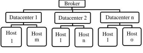
In this work, our system comprises number of distributed serving nodes and users that can change their geographic location with time i. e. experiment will be performed on heterogeneous system. To present working in hierarchical manner, we choose three level architecture as shown in figure 1[6]. The first level of architecture is Broker level; its main task is datacenter selection. Whenever a request arrives broker select the datacenter on the basis of some parameter for example, least latency from user or minimum load on data center. The next level that is second level of architecture is the data center level, its main task to decide which host will handle the request. And the third and last level is host level where virtual machines are created. Actual processing is done by virtual machine.

Fig 1: Three level system architecture

3.

CLASSIFICATION OF LOAD

BALANCING ALGORITHM

Cloud computing enables shared servers to provide resources, software for services on demand with high interoperability, scalability and reliability [7]. There is some technical challenges which are needs to be tackled before fully utilizing these benefits include resource provisioning, efficient resource consuming and system reliability. Load balancing is mainly implemented for satisfying SLA (Service Level Agreement). Load balancing is a technique to manage the resources of a node for their better utilization and user satisfaction.

It uses the concept of distributed computing in a way that it distributed the work load equally across all available computers for the fast processing and better performance. To calculate load on a node, following parameter is required; cost, response time and number of connections. Load balancing algorithms are classified in two categories: Static and Dynamic as shown in the figure 2[8].

3.1

Static Load balancing

Here we consider static information of system for the selection of least loaded node. Its performance is better in terms of complexity issue, but compromises with the result as decision is made on statically gathered data. Static load balancing is further divided into two categories as Distributed and Centralized.

In distributed static Load balancing (DSLB) approach, the final decision is made by comprehending decision of all individuals however there are many decision makers, while in centralized static load balancing (CSLB) technique, there is a controller called centralized controller that incorporates decisions of all decision makers. Distributed policies are also divided into two more categories which are co-operative and non co-operative policies.

Decision makers co-operate with each other for decision making in Co-operative policies as they have common goals. Their common goals are reduction of response time, cost incurred for processing requests and increasing throughput.

In non co-operative policies all decision makers have different goals to meet so they take independent decisions to reach an optimized and best solution for defined goals. There is only one decision maker in global static load balancing that optimizes the expected run time of entire system for all jobs.

3.2

Dynamic Load balancing

Here in this load balancing, current system state is important parameter while making decisions. Although dynamic load balancing has higher run rime complexity then static one but dynamic load balancing technique has better performance report as it takes into account the current load of system for choosing next datacenter to serve the request. This will definitely provide an optimized solution for that state of system.

Dynamic load balancing is bifurcated as Centralized and distributed. In centralized policy, there is a central computer that maintains a global state of system based on collected information and all the decisions are made based on that central computer. The only drawback with this approach is the central computer which acts as bottleneck with increase in number of computers.

Distributed load balancing approach is further divided as sender and receiver initiated and symmetrically initiated. In sender initiated approach, for processing the request is sent from heavily loaded node to lightly loaded node. Sender is identified as a node, if it accepts the next request which will exceeds its threshold level.

In receiver initiated approach, lightly loaded nodes share some load from heavily loaded nodes using request. In symmetrically initiated approach, both sender and receiver starts load balancing process. There is switching between sender and receiver initiated load balancing on the basis of load behavior as it oscillates between upper and lower threshold.

4.

RELATED WORK

Sundaram et. al., Sharma et. al., and Teo et. al. have introduced various load balancing tactics in their work which include: Round Robin, weighted round-robin, shortest expected delay, least-connection and weighted least connection [9] [10] [11]. Round Robin [12] load balancing algorithm employs time sharing between datacenters. A time quantum or time slice is defined and is allotted to all datacenters one by one. Controller keeps the datacenter ID of currently allotted time slot. Whenever a new request arrives, it is forwarded to datacenter after referring controller. It is traditional and earliest known approach and hence not very effective in balancing load as requests may have different resource requirements and size so despite of having nearly equal number of requests, all datacenters may differ widely in there load.

Weighted Round Robin load balancing technique is one in which weight is allotted to datacenters which helps in taking decision for choosing datacenter for current request. For weight allotment, they have considered various parameters like capacity of server, distance from user and many more. This approach follows principle of basic Round Robin algorithm with weight considerations. It is much better than pure round-robin and assigned higher weights to servers with better performance, thus making them more likely to be chosen results in improved system performance.

Least Connection load balancing algorithm is one in which datacenter which have to serve the request is chosen on the Broker

Datacenter 1

Host 1

Host m

Datacenter 2

Host 1

Host n

Datacenter n

Host 1

basis of number of connections linked to that datacenter. Datacenter with least number of connections implies that it is serving least number of requests so that datacenter is chosen to serve next request. It dynamically counts the connections which are linked to each server and reports the one with least count. Least connection load balancing algorithm faces problem in case two or more datacenters have same number of connections. For tiebreaking “weighted least connection” load balancing approach has been used. In this weight is allotted to each datacenter on the basis of remaining capacity and one with more weight is chosen to serve the request. It also count connections of each server but returns appropriate server based on the result of multiplication of a server weight and its connection count. In shortest expected delay load balancing approach, whenever a request arrives expected delay is calculated for all available datacenters, and the one which gives minimum expected delay will be chosen to serve the request. Here delay is a variable quantity that depends on various parameters like actual distance between datacenter and user, processing time for serving this request at datacenter and many more. It keeps record of previous response time taken by each server and returns the quickest one as the next appropriate server. All tactics mentioned above gives load to that datacenter which is least loaded, calculated on the basis of already issued workload to them but have not shown any concern about remaining capacity of server. It is totally unfair as two servers with same workload may widely differ in their capacity to consume more loads depending on their total capacity. Only way to avoid this scenario is to assume homogeneous environment as there all datacenters with same load have same remaining capacity but this is not a practical solution. Thus researchers now start focusing on load balancing algorithms that can work smoothly in heterogeneous environment.

Some other load balancing algorithm includes server load-based algorithm [13] and hash-load-based algorithms [14] [15]. Now a day’s load balancing is not confined to just server but start taking into account network links and other parameters for providing better results. Buyya and Pathan have their work published in the field of network load balancing for content delivery systems [16]. Dynamic load balancing for content delivery system chooses nodes on the basis of current system condition [17] [18]. While static load balancing for these systems use some heuristics for selecting nodes [19]. Load balancing can be performed at different levels like (i) broker level-for choosing efficient datacenter, (ii) datacenter level-for choosing efficient host at particular datacenter to serve the request and (iii) host level- for choosing efficient virtual machine to finally process the request. In this paper, we focus on broker level load balancing technique.

4.1

Broker Level Load Balancing

Algorithms

Some of the broker level load-balancing algorithms are Service proximity based routing [20], performance optimized routing [20] and cloud based multimedia load balancing [21].

4.1.1

Service proximity based routing load

balancing algorithm

In this policy a table is maintained that keeps list of all available datacenters. Whenever there is new request, service broker proximity server queries datacenter controller of destination which has the sole responsibility of returning back datacenter ID where request is to be processed. Initially datacenter controller finds the region from where request is generated. Now a list is prepared that keep datacenter IDs

lying in the same region as user in ascending order of their latency with user. Now request is sent to first datacenter in this list.

Drawback with this policy is consideration of only one parameter i.e. latency for choosing datacenter to serve the request. It is unaware of the actual load on that datacenter, a deciding parameter for response time calculation. Thus this is not the best choice for efficient load balancing.

4.1.2

Performance

optimized

routing

load

balancing algorithm

In this policy whenever a user request arrives, it find datacenters which are in the same region as the user. Now estimated response time for all those datacenters is calculated, and request is given to datacenter with minimum estimated value of response time.

Drawback of this method is that response time is calculated on the basis of processing time taken by the datacenter for serving previous request. It is not an effective way of calculating estimated response time for present request, as it may differ from previous one in some parameter like length which is deciding factor in response time calculation.

4.1.3

Cloud Based Multimedia Load Balancing

(CMLB) algorithm

Assumptions –

[1] Dynamically changing network topology- user and datacenters can change their geographic location.

[2] Homogeneous configuration for datacenters.

Steps-

[1] On arrival of new user request network link latency of user from each landmark node is calculated.

[2] Order of user from each landmark node is calculated.

[3] Similarly order of all available datacenters from each landmark nodes is calculated.

[4] Now Compare order of user with all datacenters, if matched then place all those in a list. Now load is calculated for all datacenters in this list in accordance with the following formula-

(1)

Where lij = Load of ith datacenter at the time of jth request. K= set of hosts in datacenter

Uik = Host utilization, 1 for on host and 0 for power-off host

Sik = Host capacity

[5] Next step is to calculate cost of each link from user to datacenters, for which load is calculated by this formula

(2)

Now choose datacenter with minimum calculated cost to handle the request.

5.

PROPOSED WORK

In this section, we have draw attention about the drawback of the Cloud Based Multimedia Load Balancing (CMLB) algorithm and at the same time suggested the improvement which is to be carried out in our proposed algorithm improved load balancing technique for multimedia system called ILBTM.

5.1

Drawback of CMLB and improvement

carried out in proposed algorithm ILBTM

[1] CMLB considers homogeneous datacenter configuration provide simplicity in calculation, but in real world datacenters have heterogeneous configuration. In our proposed work, we have considered heterogeneous environment.

[2] If no datacenter comes in the same region as the user, then said request is rejected and therefore degrades the throughput in CMLB. In our proposed algorithm, we have given such requests to some datacenter. However, it is not in same region but can fulfill the request in given SLA limit.

[3] In CMLB, Latency is the main parameter for calculation of network proximity and value is estimated on the basis of distance between user and datacenter. In our work, we have taken one more parameter i.e. bandwidth for calculation of latency. [4] Load calculation considers only one parameter i.e.

number of processing elements for calculating server capacity which leads to failure of virtual machine allotment due to some other parameters like RAM, Storage capacity etc resulting in more delay and thus larger response time in case of CMLB. Whereas, our proposed algorithm first check availability of RAM at host before allotting virtual machine and therefore decreasing chance of failure after allotment.

5.2

Assumptions

[1] Dynamically changing network topology - users and datacenters can change their geographic location. [2] Users and datacenters are assumed to be steady

during processing of a request. However, they are mobile.

[3] Each user request is served by exactly one virtual machine.

[4] We consider two landmark nodes for distance calculation in our work.

We propose improved load balancing technique for multimedia system called ILBTM in cloud environment to minimize response time. To begin with this algorithm, we have to find the order of user and datacenter with respect to landmark nodes. For this ordering, we use a binning scheme and for that purpose latency of user with each landmark is found and kept in a bin which is a collection of some values. For example, if distance between user and landmark nodes is 40 and 7 respectively then we can quantify these values by giving them an order like 0 for distance between 0 to 30, 1 for distance between 31 to 60 and 2 for distance above 60. So order of user with reference to landmark locations will be (1,

0), now datacenters having same order as user will be kept in same bin.

To present the work we consider set of datacenters that serve the request denoted as Ndc, set of users that generate request denoted as Nuser and set of links between Ndc and Nuser denoted by E. Now we have to calculate

Cost in terms of response time for link between user and particular datacenter, which finally serves the request. This calculation considers current load on datacenter (L) and data transmission delay (T).

Cost of link(C) can be calculated as Cost of link (C) = T*L (3) Where T= Data transmission delay L= Current load on datacenter

Data transmission delay (T) is calculated as Ttotal= Tlatency + Ttransfer (4)

Tlatency= Dact / BW (5)

Where Dact = Actual distance between user and datacenter BW= Available bandwidth

Ttransfer = Size of single request/ Available Bandwidth (6)

Load on a datacenter is calculated as

(7)

Where Rpe= required processing element

Tpe= Total processing element

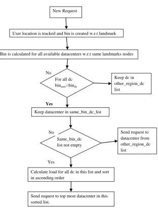
Fig 2: Flow chart for proposed methodology

Initially, we try to fetch location of request generator i. e. user. Then, we find distance between user location and landmark nodes. After quantifying this distance with binning scheme, we keep this order in an array called bin-user. Similarly, we calculate order of all available datacenters and store them in an array named bin-dc. Now check is applied, which filters out all datacenters that matches with user order. Matched datacenter ID’s are kept in a list called same_bin_dc_list and unmatched will be kept in a list denoted as other_region_dc list. After this, load is calculated for all datacenters in same_bin_dc_list and request is allotted to one with minimum load. In case, same_bin_dc_list is empty, it means there is no datacenter available in user region to serve the request. In such situation load is calculated for datacenters from other_region_dc list and request is allotted to minimum loaded datacenter among them without violating SLA. ILBTM is a load balancing algorithm that serves multimedia requests in minimum possible time. This algorithm helps us in finding minimum loaded datacenter for allocation of request. Whenever a new request arrives, first we find region from where request is generated. Then we check whether datacenter and user belong to same region or not. If they belong to same region then request is allotted to minimum loaded datacenter which has minimum calculated cost. Cost calculation is

carried out with the help of eq. (3). If there is no datacenter in same region as user, then request is served by datacenter of other region.

6.

PROPOSED ALGORITHM- ILBTM

1. for all available datacenters do

2. Calculate order of datacenters with respect to landmark nodes.

3. end for

4. for each user request do

5. Find order of user from landmark nodes. 6. for all datacenters currently available do 7. if order-user= order-datacenter then 8. Calculate data transmission delay (T) 9. Calculate current load on system (L) 10. Calculate Cost (C) = T*L

11. else

12. Cost (C) = MAXload

Yes

No

Calculate load for all dc in this list and sort in ascending order

Same_bin_dc list not empty

Keep datacenter in same_bin_dc_list New Request

User location is tracked and bin is created w.r.t landmark

nodes.

Bin is calculated for all available datacenters w.r.t same landmarksnodes

For all dc binuser=bindc

Keep dc in other_region_dc list

Yes

Send request to top most datacenter in this sorted list.

Send request to datacenter from other_region_dc list

13. end if 14. end for

15. Choose datacenter which has minimum cost value 16. end for

7.

SIMULATION CONFIGURATION

AND RESULTS

For testing this algorithm we have used Cloudsim simulator toolkit. A hypothetical configuration has been generated on the basis of results of reference taken for this work.

7.1

Simulation configuration

In this work we have used heterogeneous environment, thus have variable configuration for datacenters, hosts and virtual machines. Table 1 shows datacenter configuration. We have simulated 20 datacenters with variable number of hosts (ranges from 4 to 6) and processing elements (varies from 24 to 27). Table 2 gives configuration of host in a datacenter. Each host differs from other on the basis of two parameters namely (i) RAM capacity and (ii) number of processing elements. These parameters have direct impact on number of requests that a host can fulfill successfully. Table 3 gives configuration of virtual machine. Response time of any request depends mainly on VM’s MIPS i.e. how many instructions a VM can process per second. Response time will be less for VM with large MIPS. In this work we have taken MIPS value from 2000 to 5000.

Table 1. Configuration of Datacenters

Object Name

Number of replicas

Number of

host in each Datacenter

Total processing element in each datacenter

Datacenter 20 40-50 24-28

Table 2. Configuration of Hosts in each datacenter Object

name

RAM capacity Number of processing

elements

Host 2000-5000 5-7

Table 3 Configuration of Virtual machines

Object name

Total number

user in

simulation

Required Processing element

Million instructions per second

Virtual Machine

5-40 1 2000-5000

7.2

Simulation Result and Analysis

Experiment with specific simulation configuration is repeated 5 times to obtain the consistency in results. In our experiment, we have considered response time and processing time matrix for performance measurement. To obtain the results, we test our algorithm initially with 5 user requests from different geographic location to datacenter location generated once for

each set of request, then for 10 user requests with same scenario and so on in the multiples of 5 up to 50 user requests.

7.2.1

Comparison of Response Time

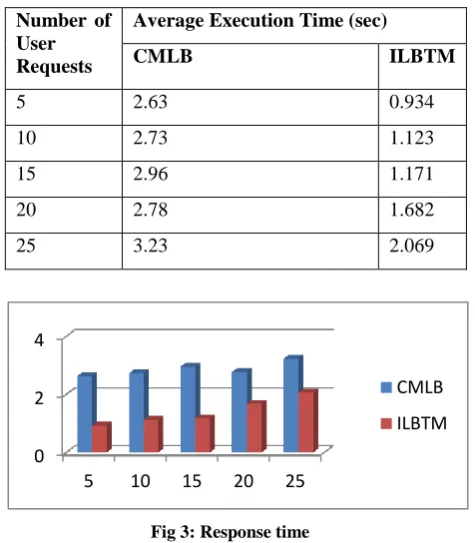
Effectiveness of Proposed algorithm (ILBTM) can be measured in terms of response time with number of user requests. Figure 4 shows the comparison between ILBTM and CMLB which proves that our proposed method outperforms the existing one by notably lowering down response time of the system. As stated in literature [19] by H.Wen, CMLB already surpassed the results of other traditional algorithms like Round Robin and number of connection to give better response time. Variation of Average response time with increasing number of user requests for CMLB and ILBTM is presented in Table 4 below:

Table 4: Average Execution Time

Number of User Requests

Average Execution Time (sec)

CMLB ILBTM

5 2.63 0.934

10 2.73 1.123

15 2.96 1.171

20 2.78 1.682

25 3.23 2.069

Fig 3: Response time

7.2.2

Effect of Cloud Environment

Since CMLB is operational in Homogeneous Cloud environment, it had same configuration for all datacenters, hosts, VMs and requests. This result in equal processing time for all arriving requests at server, but it is far from real cloud scenario, which is heterogeneous in nature. Hence in this paper proposed algorithm ILBTM, we have considered this issue by assigning distinct configuration for all entities. In this paper proposed method also provide better throughput than CMLB approach because we had tried to avoid request rejection. It is the issue that was not handled by CMLB. In CMLB approach, if requesting region do not have any datacenter in same region then that request is rejected. But in this paper serve these requests by allocating them on datacenters of some other regions. In this paper not considered migration in because migration takes time, which will eventually increase response time of the request.

0 2 4

5 10 15 20 25

CMLB

8.

CONCLUSION AND FUTURE WORK

In this paper, proposed a balancing technique for multimedia system called ILBTM in heterogeneous cloud environment considering dynamic network topology. Using this algorithm, user can effectively perform resource allocation and QoS provisioning for multimedia systems. In this experimental set up, used three level cloud architecture for better understanding of cloud working. Experimental results show that proposed approach outperforms existing algorithms in multimedia load balancing.

Although proposed algorithm provides good result for response time, but there is some scope to improve its efficiency by trying some different method of load calculation. It may consider more parameters than just number of CPUs and available RAM for calculation of load. Hence, in future one can try to add some more parameters for load calculation to improve the results.

9.

REFERENCES

[1] Jie Tao, Holger Marten, David Kramer and Wolfgang Karl, “An Intuitive Framework for Accessing Computing Clouds”, ELSEVIER International Conference on Computational Science (ICCS), pp. 2049–2057, April 2011.

[2] Tarun Goyal, Ajit Singh, Aakansha Agrawal, “Cloudsim: simulator for cloud computing infrastructure and modeling”, ELSEVIER International Conference on modeling, optimization and computing (ICMOC), vol. 38, pp. 3566-3572, 2012.

[3] D. Lea, “Concurrent Programming in JavaTM: Design Principles and Patterns”, Second Edition, Oct. 1999. [4] W. Hui; C. Lin; Y. Yang, “Mediacloud: a new paradigm

of multimedia computing”, KSII Transactions on Internet & Information Systems, vol. 6 issue 4, pp. 1153, April 2012.

[5] Rodrigo N. Calheiros, Rajiv Ranjan, César A. F. De Rose, and Rajkumar Buyya, “Cloudsim: a toolkit for modeling and simulation of cloud computing environments and evaluation of resource provisioning algorithms”, ACM journal of Software-Practice & Experience, vol.41 issue 1, pp. 23-50, Jan. 2011. [6] S. Wang, K. Yan, W. Liao and S. Wang, “Towards a

Load Balancing in a three-level cloud computing network”, 3rd IEEE International Conference on Computer Science and Information Technology (ICCSIT), vol. 1, pp. 108-113, 2010.

[7] R. Lee, B. Jeng, “Load-Balancing Tactics in Cloud”, IEEE International Conference on Cyber-Enabled Distributed Computing and Knowledge Discovery, pp. 447-454, 2011.

[8] T. Casavant and J.G Kuhl, “Taxonomy of scheduling in general-purpose distributed computing systems”, IEEE Transaction on Software Engg., vol. 14, issue 2, pp. 141-154, Feb. 1988.

[9] C. Sundaram, Y. Narahari, “Analysis of dynamic load balancing strategies using a combination of stochastic

petri nets and queuing networks”, SPRINGERLINK Application and Theory of Petri Nets: Lecture Notes in Computer Science, vol. 691, pp. 397-414, 1993.

[10] Saeed Iqbal, Graham F. Carey, “Performance analysis of dynamic load balancing algorithms with variable number of processors”, ACM Journal of Parallel and Distributed Computing, vol. 65, pp. 934-948, Aug 2005.

Jie Tao, Holger Marten, David Kramer and Wolfgang Karl, “An Intuitive Framework for Accessing Computing Clouds”, ELSEVIER International Conference on Computational Science (ICCS), pp. 2049–2057, April 2011.

[11] Jie Tao, Holger Marten, David Kramer and Wolfgang Karl, “An Intuitive Framework for Accessing Computing Clouds”, ELSEVIER International Conference on Computational Science (ICCS), pp. 2049–2057, April 2011.

[12] Tarun Goyal, Ajit Singh, Aakansha Agrawal, “Cloudsim: simulator for cloud computing infrastructure and modeling”, ELSEVIER International Conference on modeling, optimization and computing (ICMOC), vol. 38, pp. 3566-3572, 2012.

[13] D. Lea, “Concurrent Programming in JavaTM: Design Principles and Patterns”, Second Edition, Oct. 1999. [14] W. Hui; C. Lin; Y. Yang, “Mediacloud: a new paradigm

of multimedia computing”, KSII Transactions on Internet & Information Systems, vol. 6 issue 4, pp. 1153, April 2012.

[15] Rodrigo N. Calheiros, Rajiv Ranjan, César A. F. De Rose, and Rajkumar Buyya, “CloudSim: a toolkit for modeling and simulation of cloud computing environments and evaluation of resource provisioning algorithms”, ACM journal of Software-Practice & Experience, vol.41 issue 1, pp. 23-50, Jan. 2011. [16] S. Wang, K. Yan, W. Liao and S. Wang, “Towards a

Load Balancing in a three-level cloud computing network”, 3rd IEEE International Conference on Computer Science and Information Technology (ICCSIT), vol. 1, pp. 108-113, 2010.

[17] R. Lee, B. Jeng, “Load-Balancing Tactics in Cloud”, IEEE International Conference on Cyber-Enabled Distributed Computing and Knowledge Discovery, pp. 447-454, 2011.

[18] T. Casavant and J.G Kuhl, “Taxonomy of scheduling in general-purpose distributed computing systems”, IEEE Transaction on Software Engg., vol. 14, issue 2, pp. 141-154, Feb. 1988.

[19] C. Sundaram, Y. Narahari, “Analysis of dynamic load balancing strategies using a combination of stochastic petri nets and queuing networks”, SPRINGERLINK Application and Theory of Petri Nets: Lecture Notes in Computer Science, vol. 691, pp. 397-414, 1993.