Enhanced process development using automated continuous reactors by self optimisation algorithms and statistical empirical modelling

Accepted Manuscript

Enhanced process development using automated continuous reactors by self-optimisation algorithms and statistical empirical modelling

Mohammed I. Jeraal, Nicholas Holmes, Geoffrey R. Akien, Richard A. Bourne

PII: S0040-4020(18)30221-7

DOI: 10.1016/j.tet.2018.02.061 Reference: TET 29332

To appear in: Tetrahedron

Received Date: 23 October 2017 Revised Date: 22 February 2018 Accepted Date: 24 February 2018

Please cite this article as: Jeraal MI, Holmes N, Akien GR, Bourne RA, Enhanced process development using automated continuous reactors by self-optimisation algorithms and statistical empirical modelling,

Tetrahedron (2018), doi: 10.1016/j.tet.2018.02.061.

M

AN

US

CR

IP

T

AC

CE

PT

ED

Graphical Abstract

Enhanced process development using automated

continuous reactors by self-optimisation algorithms and

statistical empirical modelling

Mohammed I. Jeraal,1 Nicholas Holmes,1 Geoffrey R. Akien1,2 and Richard A. Bourne*1

Address: 1Institute of Process Research and Development, School of Chemistry & School of

Chemical and Process Engineering, University of Leeds, Leeds, LS2 9JT, UK; and

2

Department of Chemistry, Faraday Building, Lancaster University, Lancaster, LA1 4YB, UK

* Corresponding author

Email: Richard A. Bourne – [email protected]

Abstract

Reaction optimisation and understanding is fundamental for process development and is

M

AN

US

CR

IP

T

AC

CE

PT

ED

experimental design as a tandem approach to reaction optimisation. A Claisen-Schmidt

condensation was optimised using a branch and fit minimising algorithm, with the resulting

data being used to fit a response surface model. The model was then applied to find new

responses for different metrics, highlighting the most important for process development

purposes.

Keywords

self-optimisation; design of experiments; Clasien-Schmidt condensation; reaction metrics;

process development, flow chemistry

Introduction

Traditional univarient optimisation of a chemical reaction involves the systematic and

sequential optimisation of each individual reaction parameter until an optimum is found.

While the execution is simple, the data will not account for interactions between reaction

parameters.1 Design of experiments (DoE) conversely uses statistical calculations to screen

reactions and generate a polynomial model over a constrained area of experimental space. The

model can highlight the key parameters and interactions that affect changes in the desired

response, as well as predicting new responses depending on the model’s design. The

methodology is commonly utilised in the pharmaceutical industry, particularly for reactions

with poor yield, inconsistent output or unexpected results upon scale up.2 DoE is a very

powerful tool and it can show where improvements in operating conditions can be made to

deliver a more consistent and reliable product with respect to the optimisation target.

One of the disadvantages of DoE arises when there are a large number of parameters requiring

M

AN

US

CR

IP

T

AC

CE

PT

ED

increasing number of experimental parameters. Often this number can be too large to explore

the system efficiently, so a fractional factorial design is implemented to reduce the number of

experiments. The disadvantage with this approach is that at least one parameter is confounded

with an interaction, thus increasing the complexity of the model analysis. It is also very

important that the correct limits are chosen for each parameter to ensure that there are no

sudden changes in response and a good polynomial fit can be achieved. Furthermore,

additional experiments might be required to verify a response, deconvolute interactions or

determine the robustness of optimum conditions.

Self-optimisation is a technique that could remove the problems associated with DoE whilst

still obtaining the important information about key parameters and interactions. A

self-optimising reactor combines on-line analysis with an adaptive feedback loop and minimizing

algorithm to autonomously execute reactions, obtain the respective yields and ultimately

optimise a chemical process without user intervention. 3-8 The algorithm typically generates a

cluster of points around an optimum, therefore increasing the robustness of proposed optimal

conditions.

The recent popularity of self-optimisation is increasing but its use in industrial chemical

processes is severely limited.9 A continuous self-optimising reactor will benefit from the

numerous advantages of flow reactors including high surface area to volume ratios, safer

operation of hazardous materials, improved mixing, faster kinetics and easier access to

automated processes.10-13

The main disadvantage with self-optimisation is that new experiments need to be physically

executed to optimise for a new target or different chemical compound. If DoE has already

been carried out, new models for different responses can be calculated without complication

or increased experimentation.

This paper attempts to combine these two optimisation techniques in parallel. A

M

AN

US

CR

IP

T

AC

CE

PT

ED

chemical space through an exploratory algorithm, whilst a response surface model (RSM) will

permit the prediction of new responses using the experimental data.

Results and Discussion

Self-optimising reactors have been designed using a variety of analytical techniques including

IR14-16 and NMR spectroscopy17, mass spectrometry16,18, gas19-22 and liquid23,24

chromatography. In this paper, a feedback-controlled flow reactor, equipped with an at-line

HPLC system, is used to provide fast separation and quantification of the desired compounds.

Through the combined implementation of a variable wavelength UV detector and

microvolume sample injector, automated optimisations were executed at the mesoscale with

the direct injection of reaction mixture into the HPLC column, thus negating the need for

dilution prior to analysis. The optimisation target was the minor product of a Claisen-Schmidt

condensation between acetone (1) and benzaldehyde (2) to form the desired product,

benzylideneacetone (3) (Scheme 1).25 Strict control over the reaction parameters was required

to prevent 3 reacting to form dibenzylideneacetone (DBA) (4) and acetone polymerization,

M

AN

US

CR

IP

T

AC

CE

PT

ED

Scheme 1: Claisen-Schmidt condensation between acetone (1) and benzaldehyde (2) to form

the desired benzylideneacetone (3) and undesired benzylideneacetone (4). Acetone can also

undergo self-condensation to form mesityl oxide (5), as well as the subsequent polymer.

A gradient HPLC method at 254 nm was developed to quantify compounds of interest. While

adequate separation between species was achieved, preliminary HPLC calibrations resulted in

a non-linear response for 2 and 3 at the reference wavelength of 254 nm. UV spectra of both

compounds were obtained to determine the wavelengths at which each species could be

quantified, without saturating the detector (Figure 1). The HPLC method was consequently

modified to momentarily switch to 295 nm and 333 nm, when compounds 2 and 3 were

respectively eluted, to ensure the detector would not be saturated during optimisation. This

new method allowed linear calibrations of species 2-5.

Figure 1: UV absorption spectra of benzaldehyde (2) and benzylideneacetone (3) in ethanol

between 190 and 400 nm. Dashed lines indicate wavelengths selected for variable wavelength

M

AN

US

CR

IP

T

AC

CE

PT

ED

All components were monitored and controlled via a bespoke MATLAB based software

package (Reaction setup is shown Figure 6). The flow rates of the three reagent pumps and

reactor temperature were varied to maximise the yield of 3. Table 1 displays the optimisation

limits for the four reaction variables. Acetone flow was controlled relative to 2 to ensure it

was always in excess, while the temperature was limited to 80°C after initial experiments

exhibited polymer formation beyond this. While previous literature and preliminary

experiments can be used to constrain the experimental space and speed up the optimisation

process, the algorithm is also capable of optimising within the entire operating range of the

equipment being utilised. This capability is particularly advantageous when no prior

knowledge of a chemical process is available.

The algorithm used for the optimisation was SNOBFIT, a constrained branch and fit function

that locates optima by fitting polynomials to the response of experimental data points.26

During an optimisation it focuses on locating optimal conditions, whilst simultaneously

exploring empty space to prevent premature termination at local optima. In the event of

multiple optima within a chemical system, the algorithm is capable of exploring both regions

of experimental space within a single experiment.

Table 1: Parameter limits for the automated optimisation to maximise yield of 3

Reaction

Variable

Benzaldehyde 2 Flow /

mmol min-1 a

NaOH Flow /

mmol min-1 b

Acetone Flow /

mol. equivalent.c

Temperature / °C

Limits 0.4 – 2.0 0.04 – 0.25 1 – 7 10 – 80

a

1.95 M solution in ethanol with 0.0325 M biphenyl internal standard; b0.2 M solution in

M

AN

US

CR

IP

T

AC

CE

PT

ED

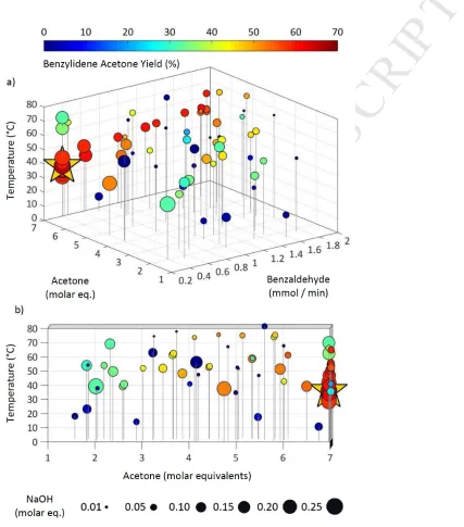
The optimisation cycle was repeated until a total of 70 experiments had been executed. The

results (Figure 2) indicate that an optimum yield of 66.0% was achieved at a benzaldehyde (2)

flow rate of 0.4 mmol/min, with 7 molar equivalents of acetone and a reactor temperature of

35.8 °C. The catalyst concentration of 0.25 M is also displayed in molar equivalents relative

to benzaldehyde to ease comparability between runs. Because the catalyst concentration was

regulated in mmol/min (Table 1), the algorithm minimised the flow rate of benzaldehyde to

0.4 mmol/min, whilst maximising the catalyst flow rate to 0.25 mmol/min, to achieve this

maximum equivalence. While the cluster of high yield experiments surrounding the optimum

were all executed at maximum NaOH equivalence, there are other experiments exhibiting

yields of around 60%, with much lower NaOH equivalents, which suggests that catalyst

concentration may not be the most significant yield limiting factor in this reaction. Following

the data points along the y-axis suggests there is some dependence on acetone concentration.

This is better appreciated when the data is viewed along the y-axis (Figure 2b) where this is a

clear correlation between acetone equivalence and yield.

There is an interaction between the benzaldehyde and NaOH flow rates and temperature,

which can be observed through the points at maximum acetone equivalence. As the flow rate

of benzaldehyde (2) increases, NaOH decreases in order to accommodate for the decrease in

residence time. This is paired with an increase in temperature to achieve higher yields at

lower catalyst loadings. This all contributes to a large area of points resembling a cliff edge at

the border of the experimental space.

As predicted, formation of DBA (4) increases at lower acetone concentrations with a

maximum yield occurring at 3.1 molar equivalences. Below this concentration, formation of

ketone 3 may be hindered by a reduced rate of acetone enolate formation.27

The residence time was calculated for each set of conditions to determine the point at which

the sample eluting from reactor, was representative of the preset experimental parameters.

M

AN

US

CR

IP

T

AC

CE

PT

ED

experiments across this range exhibited yields in excess of 60%, residence time was not

deemed to have a significant impact on the yield of 3. However, for chemical processes where

a given optimisation target is dependent on residence time, the system autonomously

optimises this parameter within the confines of the flow rate limits.

Figure 2: a): Each point represents one of the experiments executed during the optimisation.

Graph displays five variables as follows: (x) molar flow rate of benzaldehyde, (y) molar

M

AN

US

CR

IP

T

AC

CE

PT

ED

NaOH catalyst concentration in each run. The colour of each point represents the yield (%) of

3 in relation to 2. A maximum yield of 66.0% was achieved, the conditions of which are

highlighted by the star. b) Identical to a) but rotated to depict data as viewed along the y-axis.

The formation of other UV active species which were not calibrated prior to the optimisation

could also be monitored because a full HPLC chromatogram was collected for each set of

reaction conditions. Any compounds of interest could be characterised against reference

materials and subsequently quantified following a HPLC calibration. The HPLC method

switches to 254 nm outside regions of interest to maximise absorption resulting from ancillary

organic species. This, coupled with the direct injection of sample into the instrument, ensures

that even low level products can be detected.

The concentration of any compound can later be increased with the corresponding yield

optimisation.22 The existing responses can be used as a starting point to limit the number of

experiments required for completion, but additional optimisations ultimately result in an

increase of time and resource. A better methodology could be to predict where unknown

compounds have the highest yields and then carry out yield optimisations in a smaller

operating window around that point. This can be achieved by fitting a response surface to the

existing data.

Response surfaces were obtained for compounds 2, 3 and 4 using a multiple linear regression

(MLR) fit.28 Models were first generated by including all square and interaction terms, then

removing non-significant coefficients for which the calculated error potentially equalled zero.

Next, experiments were removed that fell beyond ± 2.5 standard deviations (SD) on a normal

probability residual plot. Outliers are typically removed (or repeated) if they fall outside of ±4

SD but the lower tolerance in this instance allowed for a better fit and greater predictability.

The lowest number of experiments in a model was 65, which was in excess of the requirement

M

AN

US

CR

IP

T

AC

CE

PT

ED

experiments was therefore not deemed to numerically compromise the model. A good fit was

achieved for all three compounds with R2 values of 0.73 (2), 0.91 (3) and 0.85 (4). These

models also showed a moderate level of predictability with Q2 values of 0.66 (2), 0.86 (3) and

0.78 (4).

The models were subsequently used to predict an optimum yield by maximising the response

of 3 (minimum tolerance 65%) and minimising 2 and 4 (maximum tolerance 5%). Conditions

obtained that satisfied two of those criteria were: 1.97 mol/min of 2, 4.8 molar eq. of acetone,

0.1 mmol/min of NaOH and a reactor temperature of 80 °C, generating 3 in a 61.1% yield.

These conditions do not match the optimal conditions generated by the self-optimisation, for

which the model calculates a yield of 59.5 %. Both the predicted and experimental optima are

within the error associated with HPLC analysis, indicating that there is a plateau of conditions

that generate 3 at approximately 60% yield.

Further scrutiny of the SNOBFIT optimum data point showed that there was a significant rise

in yield compared to points in close vicinity. This, coupled with the disagreement in optima

between the two techniques prompted some further experimentation to study the

reproducibility of the algorithm optimum. Three further experiments were carried out at the

optimum conditions, which generated 3 in a mean yield of 64.4% ± 0.3% (arithmetic mean ±

1 SD). This shows that the previous optimum value was possibly caused by an integration

error from HPLC analysis.

A second self-optimisation for the generation of 3 was executed to determine if yields could

be further increased by expanding on the existing experimental space. As lower acetone

equivalents previously displayed lower yields, Table 2 shows how acetone equivalence limits

were increased from 1-7 to 5-14 molar equivalents. The maximum NaOH flow rate was also

increased to 0.1 mmol/min as the optimum point was at its upper limit. Whilst the

M

AN

US

CR

IP

T

AC

CE

PT

ED

parameter limit was halved (to 1 mmol/min) to compensate for the increase in experimental

space and minimise the detriment to operating efficiency. The maximum temperature was also

reduced from 80 to 60 °C for the same reasons.

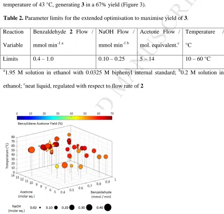
The SNOBFIT algorithm was then restarted using existing data within the new operating

conditions (Table 2). The new optimisation required 36 further experiments and produced

optimum conditions of 0.76 mmol/min of 2, 14 eq of acetone, 0.15 mmol/min of NaOH, and a

temperature of 43 °C, generating 3 in a 67% yield (Figure 3).

Table 2. Parameter limits for the extended optimisation to maximise yield of 3.

Reaction

Variable

Benzaldehyde 2 Flow /

mmol min-1 a

NaOH Flow /

mmol min-1 b

Acetone Flow /

mol. equivalent.c

Temperature /

°C

Limits 0.4 – 1.0 0.10 – 0.25 5 – 14 10 – 60 °C

a

1.95 M solution in ethanol with 0.0325 M biphenyl internal standard; b0.2 M solution in

ethanol; cneat liquid, regulated with respect to flow rate of 2

Figure 3. Plot of experiments performed during extended automated yield optimisation of

benzylideneacetone (3) via the aldol condensation of benzaldehyde (2) with acetone. The

M

AN

US

CR

IP

T

AC

CE

PT

ED

been adjusted to allow for more acetone and catalyst equivalents versus the first yield

optimisation (see Table 2). A maximum yield of 66.6% was achieved as highlighted by the

star.

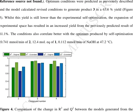
New models were fitted using the same approach and improved R2 (fit) and Q2 (predictability)

was achieved for all models using the data from the extended optimisation (Figure 4Error!

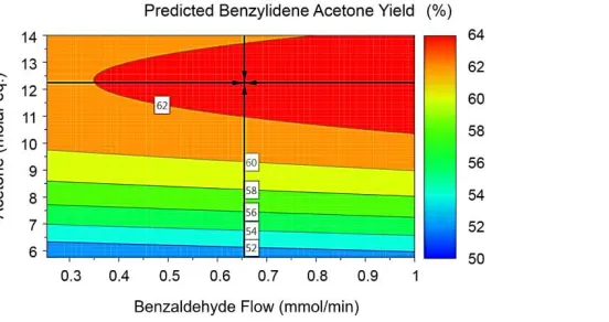
Reference source not found.). Optimum conditions were predicted as previously described

and the model calculated revised conditions to generate product 3 in a 63.6 % yield (Figure

5). Whilst this yield is still lower than the experimental self-optimisation, the expansion of

experimental space has resulted in an increased yield from the previously predicted result of

61.1%. The conditions also correlate better with the optimum produced by self-optimisation

(0.741 mmol/min of 2, 12.4 mol. eq of 1, 0.112 mmol/min of NaOH at 47.2 °C).

Figure 4. Comparison of the change in R2 and Q2 between the models generated from the

original and extended data.

2 3 4

0 0.2 0.4 0.6 0.8 1

Compound number

M

AN

US

CR

IP

T

AC

CE

PT

ED

Figure 5: Contour plot of predicted benzylideneacetone yields using original and extended

data. Optimum point with a predicted yield of 63.6% is shown by crosshair.

While it seems achievable to improve the maximum observed product 3 yield of 67% by

extending the experimental space to allow for greater acetone and hydroxide equivalents, it is

worth considering whether increasing the reagent cost in pursuit of a higher product yield

would be financially or materially efficient upon scale up of the reaction. Although yield was

the target parameter in this optimisation, previous research has demonstrated how these

systems can be utilised to optimise other metrics such as E factor, process mass intensity and

reaction productivity to improve the sustainability of a chemical process.16,23,29,30 The

advantage of a statistical model following self-optimisation means that such metric analyses

can be carried out without further practical experiments.

This ability to predict alternative metrics has been demonstrated by further fitting of the

experimental data used to create the existing models. The metrics explored in this study were

process mass intensity (PMI),31 a measure of the total chemical resource per mass unit of

product; space time yield (STY), the mass of product formed per unit volume per unit time;

M

AN

US

CR

IP

T

AC

CE

PT

ED

models for these metrics were fitted using MLR with R2 values of 0.93 (PMI), 0.92 (STY) and

0.90 (cost); and Q2 values of 0.86 (PMI), 0.86 (STY) and 0.83 (cost).

Table 3. Effect of different metrics on the product composition of compounds 2-4

Metric

target

2 / % Yield 3 / % Yield 4 / % Yield PMI STY / g L

-1 h-1

Cost / £

kg-1

Yield 3.22 65.62 3.01 18.48 633.20 33.45

PMI 4.54 47.90 6.02 13.81 614.36 27.92

STY 3.06 62.15 4.45 19.11 872.69 34.50

Cost 4.15 58.81 4.13 14.30 798.39 26.72

Yield PMIa 4.28 55.32 4.70 13.99 729.52 26.91

PMI Costb 2.96 64.81 3.66 16.35 769.93 29.57

The first column shows the metric target, responses are shown in the rows. Maximum values

are highlighted in bold, minimized values are highlighted in italics. Unformatted values

display the models’ predicted values. amaximise the yield of 3 whilst minimising the PMI;

b

minimise both PMI and cost.

Table 3 shows how the model responses change with optimum conditions for different metric

targets. The maximum yield exhibits poor responses for PMI, STY and cost, showing how

high yielding reactions can be wasteful and unproductive. The optimum response for PMI is

the least productive and for the studied metrics, predicts the lowest yield for 3 at 48%. There

is good correlation between the responses of PMI and cost for all the metric targets. This

should be expected as both are dependent on the ratio of product to substrates and reagents.

The raw material cost calculation aims to put bias on reducing the concentrations of expensive

M

AN

US

CR

IP

T

AC

CE

PT

ED

extent than lower PMI, thus indicating that raw material cost could be the most important

metric in this reaction format. This is assuming that the adoption of cheaper reagent does not

increase the reaction complexity and therefore increase the cost of work-up and purification.

Table 4. Predicted conditions for the optimum responses to different metric targets

Metric target 2 Flow / mmol

min-1

NaOH Flow /

mmol min-1

Acetone /

equivalents

Temperature /

°C

Yield 0.741 0.112 12.4 47.2

PMI 0.846 0.044 6.0 44.1

STY 1.000 0.150 13.9 42.2

Cost 0.986 0.067 9.2 47.1

Yield PMIa 0.915 0.055 7.5 45.5

PMI Costa 0.998 0.096 10.5 46.8

a

maximize the yield of 3, minimize the PMI; bminimize both PMI and cost.

The conditions for the optimal responses are shown in Table 4. The flow rate of 2 is close to

its upper limit for every target. This reduces the residence time and consequently increases the

reaction productivity (STY). The acetone equivalents are generally lower than those generated

by the yield driven self-optimisation, thus limiting the reagent waste (through PMI and cost).

Strict temperature control is required in compensation to maintain the high yields of 3, whilst

minimising risk of polymer formation.

Conclusion

The yield of a minor product in a Claisen-Schmidt condensation has been optimised using a

M

AN

US

CR

IP

T

AC

CE

PT

ED

was optimised directly at the mesoscale to produce 0.24 kg/day of the desired

benzylideneacetone, 3. Through the development of a variable wavelength HPLC method, all

organic species of interest could be quantified within their respective linear detection limits.

With the data obtained from the self-optimisation, a response surface was fitted to the main

compounds of interest in the reaction (2-4). After an analysis of the self-optimisation data and

resulting models, it was decided to execute a further optimisation in a larger chemical space.

The second experimental optimisation improved upon the yield of 3 and the increased

correlation between the new optimum and surrounding experimental points, provided a

greater range of conditions at which optimal yields could be obtained. The subsequent

statistical model of the extended optimisation also predicted similar optimal conditions.

It should be noted that the choice of algorithm in the initial self-optimisation step is critical to

achieving a good fit to the RSM. The simplex algorithm and modifications thereof,32-35 are a

popular choice in self-optimising systems.16,17,19-24 During operation, however, only

experiments with an improved predicted response will be executed, therefore negating

valuable information existing in the experimental space between the initial and optimum

points. The execution of random conditions and exploration of free space offered by

SNOBFIT provides a scatter of data, without which the additional response surface fitting

would not be possible. In this study, the increased robustness resulting from the additional

experimental points around the optimum would also have been forfeited with a simplex

approach.

In this example, the experimental optimum was identified at the edge of the initial

optimisation space. Prediction of the optimum via the statistical model was therefore

compromised due to the inability to fit a polynomial to changes induced by the cliff edge. The

experimental self-optimisation, however, freely explored the edge of the optimisation space to

M

AN

US

CR

IP

T

AC

CE

PT

ED

the superior technique for chemical process optimisation. When used in tandem, however, the

subsequent response fitting of self-optimisation data can predict the responses of different

species and even alternate metrics without additional experimentation. It therefore follows

that self-optimisation and DoE can be interdependent, rather than conflicting techniques,

which can combine to provide a wealth of information in the scale-up and process

optimisation of chemical systems.

Experimental

Automated yield optimisation: Reaction control, yield calculation and process optimisation

were under full MATLAB automation via a bespoke program utilising the SNOBFIT

optimisation algorithm. The reactor was setup as displayed in Figure 6 for HPLC calibration

and experimental yield optimisations.

Figure 6: Schematic of automated self-optimising flow reactor. Bespoke MATLAB based

control software monitored and regulated the following: flow rate and pressure of the reagent

pumps (P1, P2 & P3); temperature of the tubular reactor and activation of the sample injector.

Reagents were pumped at the specified flow rates through individual Jasco PU-980 HPLC

M

AN

US

CR

IP

T

AC

CE

PT

ED

specified temperature using a Polar Bear Plus Flow Synthesizer. A sample from each set of

conditions was acquired by a VICI Valco 4 Port Microvolume Sample Injector. HPLC

analysis was carried out by an Agilent 1100 HPLC System with G1314B Variable

Wavelength Detector. Pressure was maintained using a Jasco BP-1580 Back Pressure

Regulator and Polyflon 1/16” (OD) PTFE tubing was utilised throughout the 6.5 ml reactor.

Five sets of reaction conditions were initially selected and autonomously executed by the

software. The yields of these experiments were calculated from the HPLC response using a

biphenyl present in the reagent. Subsequent conditions were then generated by fitting yield

responses to the data using the SNOBFIT. 70 experiments were executed as 14 cycles of 5

experiments under full MATLAB automation. Following initial response fitting, an additional

36 experiments were carried as described in Table 2.

Variable wavelength HPLC Method: Calibration and optimisation analyses were executed

using an Agilent 1100 Series HPLC System equipped with a G1312A binary pump and

G1314B variable wavelength detector (VWD). Compounds were separated via an Ascentis

Express C18 column (5.0 µm particle size, 4.6 mm diameter x 50 mm length). Mobile phase

was a binary mixture of acetonitrile and water (MeCN-H2O), each containing 0.1% (v/v) of

trifluoroacetic acid. Method was gradient based with a 5:95 (v/v) MeCN-H2O starting

mixture. Concentration was immediately increased to 95:5 (v/v) MeCN-H2O via a 7 min

linear gradient, followed by an immediate decrease back to 5:95 (v/v) MeCN-H2O via a 2 min

linear gradient, where it remained for 1 min. Total run time was 10 mins at a constant flow

rate of 1.2 ml/min with a column temperature of 20 °C throughout. The absorption

wavelength of the VWD operates at base value of 254 nm. 3.4 mins into the method, the

wavelength switches to 295 nm for 0.2 mins. At 4.2 mins, there is a switch to 333 nm for 0.2

M

AN

US

CR

IP

T

AC

CE

PT

ED

Acquisition of UV spectra: 2 M solutions of 2 and 3 in ethanol were manually injected

through an Agilent 1100 HPLC System with G1314B variable wavelength detector. A UV

absorption spectrum between 190 and 400 nm was captured for each species upon elution.

HPLC Calibration: Reactor was setup as depicted in Figure 6. A solution of analyte (2.0 M)

was pumped against solvent at varying flow rates, with a total flow of 1 ml/min, to create a

10-point calibration graph. Two reactor volumes of material was eluted prior to HPLC sample

injection. Flow rates and sample injection were autonomously controlled via a MATLAB

based program.

Statistical Modelling: Multiple linear regression fits were applied to the automated

experimental results using the MODDE software package from UMetrics. Predicted responses

for the yields of compounds 2, 3 and 4, as well as reaction metrics including process mass

intensity, space time yield, and bulk cost of reagents were obtained using multiple linear

regression. Interactions with the potential of zero contribution to the measured response, as

well as individual experiments with high residual error were negated to maximise the model

fitting.

See ESI for full details on the reactor setup, HPLC method, individual parameters for the

automated yield optimisations and the statistical analysis methodology.

Acknowledgements

The authors would like to thank Rebecca Meadows, Robert Woodward and Brian Taylor from

AstraZeneca for project support, Matthew Broadbent for workshop support and Simon Barrett

and Martin Huscroft for analytical support as well as Bao Nguyen and group. NH thanks

EPSRC, AstraZeneca and University of Leeds for a DTG case funded studentship.

M

AN

US

CR

IP

T

AC

CE

PT

ED

1. Rasheed, M.; Wirth, T. Angew. Chem., Int. Ed. 2011, 50, 357-358.

2. Weissman, S. A.; Anderson, N. G. Org. Process Res. Dev. 2015, 19, 1605-1633.

3. Krishnadasan, S.; Brown, R. J. C.; deMello, A. J.; deMello, J. C. Lab on a Chip 2007, 7, 1434-1441.

4. McMullen, J. P.; Stone, M. T.; Buchwald, S. L.; Jensen, K. F. Angewandte Chemie International Edition 2010, 49, 7076-80.

5. Skilton, R. A.; Bourne, R. A.; Amara, Z.; Horvath, R.; Jin, J.; Scully, M. J.; Streng, E.; Tang, S. L. Y.; Summers, P. A.; Wang, J.; Perez, E.; Asfaw, N.; Aydos, G. L. P.; Dupont, J.; Comak, G.; George, M. W.; Poliakoff, M. Nature Chemistry 2015, 7, 1-5.

6. Fabry, D. C.; Sugiono, E.; Rueping, M. React. Chem. Eng. 2016.

7. Holmes, N.; Bourne, R. A. In Chemical Process Technology for a Sustainable Future; Letcher, T. M.; Scott, J. L.; Paterson, D. A. Eds.; RSC Publishing, 2014; pp. 28-45.

8. Sans, V.; Cronin, L. Chem. Soc. Rev. 2016, 45, 2032-2043.

9. Holmes, N.; Akien, G. R.; Blacker, A. J.; Woodward, R. L.; Meadows, R. E.; Bourne, R. A. React. Chem. Eng. 2016, 1, 366-371.

10. Hessel, V. Chem. Eng. Technol. 2009, 32, 1655-1681.

11. Wegner, J.; Ceylan, S.; Kirschning, A. Adv. Synth. Catal. 2012, 354, 17-57.

12. Ley, S. V.; Fitzpatrick, D. E.; Ingham, R. J.; Myers, R. M. Angew. Chem. Int. Ed. 2015, 54, 3449-3464.

13. Ley, S. V.; Fitzpatrick, D. E.; Myers, R. M.; Battilocchio, C.; Ingham, R. J. Angew. Chem., Int. Ed. 2015, 54, 10122-10136.

14. Skilton, R. A.; Parrott, A. J.; George, M. W.; Poliakoff, M.; Bourne, R. A. Appl. Spectrosc.

2013, 67, 1127-1131.

15. Mattrey, F.; Dolman, S.; Nyrop, J.; Skrdla, J. Am. Pharm. Rev. 2012, 15.

16. Fitzpatrick, D. E.; Battilocchio, C.; Ley, S. V. Org. Process Res. Dev. 2015, 20, 386–394. 17. Sans, V.; Porwol, L.; Dragone, V.; Cronin, L. Chem. Sci. 2015, 6, 1258-1264.

18. Holmes, N.; Akien, G. R.; Savage, R. J. D.; Stanetty, C.; Baxendale, I. R.; Blacker, A. J.; Taylor, B. A.; Woodward, R. L.; Meadows, R. E.; Bourne, R. A. React. Chem. Eng. 2016, 1, 96-100.

19. Parrott, A. J.; Bourne, R. A.; Akien, G. R.; Irvine, D. J.; Poliakoff, M. Angew. Chem., Int. Ed.

2011, 50, 3788-3792.

20. Bourne, R. A.; Skilton, R. A.; Parrott, A. J.; Irvine, D. J.; Poliakoff, M. Org. Process Res. Dev. 2011, 15, 932-938.

21. Jumbam, D. N.; Skilton, R. A.; Parrott, A. J.; Bourne, R. A.; Poliakoff, M. J. Flow Chem.

2012, 2, 24-27.

22. Amara, Z.; Streng, E. S.; Skilton, R. A.; Jin, J.; George, M. W.; Poliakoff, M. Eur. J. Org. Chem. 2015, 2015, 6141-6145.

23. McMullen, J. P.; Jensen, K. F. Org. Process Res. Dev. 2010, 14, 1169-1176.

24. McMullen, J. P.; Stone, M. T.; Buchwald, S. L.; Jensen, K. F. Angew. Chem., Int. Ed. 2010, 49, 7076-7080.

25. Drake, N. L.; Allen, P. Org. Synth. 1923, 3, 17-20.

26. Huyer, W.; Neumaier, A. ACM Trans. Math. Softw. 2008, 35, 1-25.

27. Tanaka, K.; Motomatsu, S.; Koyama, K.; Fukase, K. Tetrahedron Lett. 2008, 49, 2010-2012. 28. Umetrics MODDE; Sartorius Stedim Biotech.

29. Jumbam, D. N.; Skilton, R. A.; Parrott, A. J.; Bourne, R. A.; Poliakoff, M. Journal of Flow Chemistry 2012, 2, 24-27.

30. Skilton, R. A.; Parrott, A. J.; George, M. W.; Poliakoff, M.; Bourne, R. A. Applied Spectroscopy 2013, 67, 1127-31.

31. Jimenez-Gonzalez, C.; Ponder, C. S.; Broxterman, Q. B.; Manley, J. B. Org. Process Res. Dev. 2011, 15, 912-917.

32. Spendley, W.; Hext, G. R.; Himsworth, F. R. Technometrics 1962, 4, 441-461. 33. Nelder, J. A.; Mead, R. Comput. J. 1965, 7, 308-313.

34. Routh, M. W.; Swartz, P. A.; Denton, M. B. Anal. Chem. 1977, 49, 1422-8.