Self-Organised Direction Aware Data Partitioning Algorithm
Xiaowei Gu1, Plamen Angelov1,2*, Dmitry Kangin1 and Jose Principe3
1 School of Computing and Communications, Lancaster University Lancaster, LA1 4WA, UK. e-mail: {x.gu3, p.angelov, d.kangin}@lancaster.ac.uk
2 Honorary Professor, Technical University of Sofia, boulevard Kliment Ohridski 8, 1000, Sofia, Bulgaria 3
Computational NeuroEngineering Laboratory, Department of Electrical and Computer Engineering, University of Florida, USA. e-mail: [email protected]
Abstract: In this paper, a novel fully data-driven algorithm, named Self-Organised Direction Aware (SODA) data partitioning and forming data clouds is proposed. The proposed SODA algorithm employs an extra cosine similarity-based directional component to work together with a traditional distance metric, thus, takes the advantages of both the spatial and angular divergences. Using the nonparametric Empirical Data Analytics (EDA) operators, the proposed algorithm automatically identifies the main modes of the data pattern from the empirically observed data samples and uses them as focal points to form data clouds. A streaming data processing extension of the SODA algorithm is also proposed. This extension of the SODA algorithm is able to self-adjust the data clouds structure and parameters to follow the possibly changing data patterns and processes. Numerical examples provided as a proof of the concept illustrate the proposed algorithm as an autonomous algorithm and demonstrate its high clustering performance and computational efficiency.
Keywords: autonomous learning, nonparametric, clustering, Empirical Data Analytics (EDA), cosine similarity,
traditional distance metric.
1. Introduction
Tremendous increase in the volume and complexity of the data (streams) combined with rapid development of computing hardware capabilities requires a fundamental change of the existing data processing methods. Developing advanced data processing methods that have elements of autonomy and deal with streaming data is now becoming increasingly important for industry and data scientists alike [4], [11].
[16], [42], etc. Moreover, the parameters and thresholds that are required to be pre-defined are often problem- and sometimes user-specific, which inevitably leads to the subjective results; this is usually ignored and neglected portraying clustering and related data partitioning techniques as unsupervised.
Generally, clustering algorithms may use miscellaneous distances to measure the separation between data samples. However, the well-known Euclidean and the Mahalanobis [27], [33] distance metrics are the most frequently used ones. In some fields of study such as natural language processing (NLP), for example, the derivatives of the cosine (dis)similarity, which is a pseudo metric, are also used in the machine learning algorithms for clustering purpose [3], [38], [39]. Nevertheless, once a decision is made, only one type of distance/dissimilarity can be employed by the clustering algorithms.
Empirical Data Analytics (EDA) [5]-[7] is a recently introduced nonparametric, assumption free, fully data driven methodological framework. Unlike the traditional probability theory or statistic learning approaches [9], EDA is conducted entirely based on the empirical observation of the data alone without the need of any prior assumptions and parameters. It has to be stressed that the concept of “nonparametric” means our
algorithms is free from user- or problem- specific parameters and presumed models imposed for the data generation, but this does not mean that our algorithms do not have meta-parameters to achieve data processing.
In this paper, we introduce a new autonomous algorithm named Self-Organised Direction Aware (SODA) data partitioning. In contrast to clustering, a data partitioning algorithm firstly identifies the data distribution peaks/modes and uses them as focal points [7] to associate other points with them to form data clouds [8] that resembles Voronoi tessellation [34]. Data clouds [8] can be generalized as a special type of clusters but with many distinctive differences. They are nonparametric and their shape is not pre-defined and pre-determined by the type of the distance metric used (e.g. in traditional clustering the shape of clusters derived using the Euclidean distance is always spherical; clusters formed using Mahalanobis distance are always hyper-ellipsoidal, etc.). Data clouds directly represent the local ensemble properties of the observed data samples.
The SODA partitioning algorithm employs both a traditional distance metric and a cosine similarity based angular component. The widely used traditional distance metrics, including Euclidean, Mahalanobis, Minkowski distances, mainly measure the magnitude difference between vectors. The cosine similarity, instead, focuses on the directional similarity. The proposed algorithm that takes into consideration both the spatial and the angular divergences results in a deeper understanding of the ensemble properties of the data.
angular divergences and, based on them, discloses the ensemble properties and mutual distribution of the data. The possibility to calculate the EDA quantities incrementally enables us to propose computationally efficient algorithms.
Furthermore, a version of the SODA algorithm for streaming data is also proposed, which is capable of continuously processing data streams based on the offline processing of an initial dataset. This version enables the SODA algorithm to follow the changing data pattern in an agile manner once primed/initialised with a seed dataset. The numerical examples in this paper demonstrate that the proposed autonomous algorithm constantly outperforms the state-of-the-art methods, producing high quality clustering results and has high computational efficiency.
The remainder of this paper is organised as follows. Section 2 introduces the theoretical basis of the proposed methodology and approach. Section 3 presents the main procedure of the proposed SODA partitioning algorithm. The streaming data processing extension is described in section 4. Numerical examples and performance evaluations are given in section 5. This paper is concluded by section 6.
2. Theoretical Basis
Firstly, let us consider the real data space m
R and assume a data set/stream as
x x x1, 2, 3...
, where T,1, ,2,..., ,
m ixi xi xi m R
x is a mdimensional vector, i1, 2,3,...; m is the dimensionality; subscript i
i1, 2,3,...
indicate the time instances at which the ith data sample arrives. In real situations, data samplesobserved at different time instances may not be exactly the same, however, with a given granularity of measurement, one can always expect that the values of some data samples repeat more than ones. Therefore, within the observed data set/stream at the th
n time instance denoted by
x x1, 2,...,xn
, we also consider the setof sorted unique values of data samples
1, 2,...,
u
n
u u u ( ,1, ,2,..., , T m
i ui ui ui m R
u ) from
x x1, 2,...,xn
and the corresponding normalised numbers of repeats
1, 2,...,
u
n
f f f , where nu ( 1nu n) is the number of
unique data samples and 1
1
u
n i i
f
. The following derivations are conducted at the nth time instance as a defaultunless there is a specific declaration.
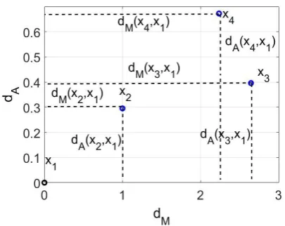
2.1. Distance/Dissimilarity Components in SODA
ii) a directional/angular component based on the cosine similarity;
and, thus, it is able to take advantage of the information extracted within a metric space and within a pseudo-metric, similarity oriented one, namely, the spatial and directional divergences.
The magnitude component can be, but is not limited to, the well-known Euclidean or Mahalanobis distances as well as other known full metric types of distances. For the clarity of the derivation, the most widely used Euclidean distance metric will be used in this paper as the magnitude component, and thus, the magnitude component is expressed as:
2, ,
1
, ; , 1, 2,...,
m
M i j i j i l j l l
d x x i j n
x x x x (1)
The angular component is based on the cosine similarity and expressed as:
,
1 cos
i, j
; , 1, 2,...,A i j
d x x x x i j n (2)
where cos
,
,i j
i j i j
x x x x
x x ,
x xi, j is the angle between xiandxj.In the Euclidean space, since , , 1 ,
m i j i l j l
l
x x
x x and xi x xi, i , the directional component
,
A i j
d x x can be rewritten as follows:
2 2
, , , , , ,
1 1 1 1
2 2 2 , , 1 ,
, 1 1
2 2
; , 1, 2,...,
1 1
2 2
m m m m
i l j l i l j l i l j l
i j l l l l
A i j
i j i j i j i j
m
j l j
i l i
l i j i j
x x x x x x
d
i j n
x x
x x x xx x x x x x x x
x x
x x x x
(3)
One can notice that, if xor y are equal to 0, thendA
x xi, j
0.genome decoding [43], spectroscopy [19], fault detection of aviation data [32], image recognition [27], [30], etc.
Fig. 1. Illustrative example of the DA plane
2.2. EDA Operators
The recently introduced Empirical Data Analytics (EDA) is an alternative methodology for machine learning which is entirely based on actual empirically observed data samples [5]-[7]. It estimates the ensemble properties of the empirically observed discrete data based on their relative proximity in the data space; thus, EDA is free from user- and problem- specific parameters and entirely data-driven.
The main EDA operators are described in [5]-[7], which are also suitable for streaming data processing. The EDA operators include:
i) Cumulative Proximity
The cumulative proximity,
of xi (i1, 2,...,n) is defined as [5]-[7]:
2
1 , n
n i i j
j d
x x x (4) where d
x xi, j
denotes the distance/dissimilarity between xiand xj.With the Euclidean component dM, the cumulative proximity can be calculated recursively as [6]:
2 2
2 1
, n
M M M M
n i M i j i n n n
j
d n X
x x x x (5) where nMis the mean of
x x1, 2,...,xn
andM n
X is the mean of
x1 2, x2 2,..., xn 2
; they can be updatedrecursively as [4]:
1 1 1
1 1
;
M M M
n n n
n
n n
2 2
1 1 1
1 1
;
M M M
n n n
n
X X X
n n
x x (7)
Using the angular component, the cumulative proximity can be rewritten as:
2 2 2 2 2 1 , 1 2 2 nA i A A A i A A
n i A i j n n n n n
j i i
n n d X
x x x x x
x x (8)
where nMis the mean of 1 2
1 2
, ,..., n n x x x
x x x and 1
A i
X (i1, 2,...,n), and similarly:
1
1 1
1
1 1
;
A A n A
n n
n n
n n
x x
x x (9) ii) Local Density
Local density D is defined as the inverse of the normalised cumulative proximity and it directly indicates the main pattern of the observed data [6], [7]. The local density, D of xi(i1, 2,...,n; nu 1) is defined as follows [6], [7]:
1
2 n n j j n i n i D n
x xx (10)
One can see that, with the Euclidean distance metric,
1 n n j j
x gets the form of [6], [7]:
2
2 1
2 n
M M M
n j n n
j
n X
x (11)For the angular component,
1 n n j j
x can be re-written as:
2
2
11 n
A A
n j n
j
n
x (12) Thus, for the case of Euclidean distance, the local density reduces to the following Cauchy type function [6], [7]:
22 1 1 M n i M i n M M n n D X x x (13)
2 2 1 1 1 A n i A i n A n D x x (14)In the proposed SODA data partitioning approach, since both components, the magnitude (metric) and the angular one are equally important, the local density of xi(i1, 2,...,n; nu 1) is defined as the sum of the metric/Euclidean-based local density ( M
n i
D x ) and the angular-based local density ( A
n iD x ):
2 22 2
1 1
1 1
1
M A
n i n i n i
M A
i n i n
M M A
n n n
D D D
X
x x x
x x
(15)
iii) Global Density
The global density is defined for unique data samples together with their corresponding numbers of repeats in the data set/stream. It has the ability of providing multi-modal distributions automatically without the need of user decisions, search/optimisation procedures or clustering algorithms. The global density of a particular unique data sample, ui (i1, 2,...,nu;nu 1) is expressed as the product of its local density and its number of repeats considered as a weighting factor [7] as follows:
G
n i i n i
D u f D u (16) As we can see from the above equations, the main EDA operators: cumulative proximity (
), local density (D) and global density ( GD ) can be updated recursively, which shows that the proposed SODA algorithm is suitable for online processing of streaming data.
3. SODA Algorithm for Data Partitioning
In this section, we will describe the proposed SODA algorithm. The main steps of the SODA algorithm include: firstly, form a number of DA planes from the observed data samples using both, the magnitude-based and angular-based densities; secondly, identify focal points; finally, use the focal points to partition the data space into data clouds. The detailed procedure of the proposed SODA partitioning algorithm is as follows.
3.1. Stage 1: Preparation
2 2
2
1 1 1 1
2
2 2
,
2
n n n n
M i j i j
i j i j M M
M n n
d d X n n
x x x x
(17)
2 2
1 1 2
1 1 2 2 2 , 1 2 n n
n n i j
A i j
i j i j
i j A
A n d d n n
x xx x x x
(18)
Then, we can obtain the global density, G
n iD u (i1, 2,...,nu) of the unique data samples
1, 2,...,
u
n
u u u
using equation (16). After the global densities of all the unique data samples are calculated, they are ranked in a descending order and renamed as
ˆ ˆ1, 2,...,ˆ
u
n
u u u .
3.2. Stage 2: DA Plane Projection
The DA projection operation begins with the unique data sample that has the highest global density, namely uˆ1. It is initially set to be the first reference, 1uˆ1, which is also the origin point of the first DA plane, denoted by P1 (L1, L is the number of existing DA planes in the data space). For the rest of the unique data samples uˆj (j2,3,...,nu), the following rule is checked sequentially:
Condition 1
ˆ ˆ
, 1 , 1
ˆ
M l j A l j
M A l j d d IF AND d d THEN P
u u
u
(19)
where l1, 2,...,L; is set to decide the granularity of the clustering results and relates to the Chebyshev inequality [37]; here 6 is used for all the datasets and problems.
If two or more DA planes satisfy Condition 1 (equation (19)) at the same time, uˆj will be assigned to the nearest of them:
1,2,...,
ˆ ˆ
, ,
arg min M l j A l j
l L M A d d i d d
u u
(20)
The meta-parameters (mean i , support/number of data samples, denoted by Si and sum of global density, denoted by Di) of the ith DA plane are being updated as follows:
1 ˆ
1 1
i
i i j
i i
S
S S
u (21a) 1
i i
ˆ G i iDn jD D u (21c) If Condition 1 is not met, uˆj is set to be a new reference and a new DA plane PL1 is set up as follows:
1
L L (22a) ˆ
L j
u (22b)1 L
S (22c)
ˆG L Dn j
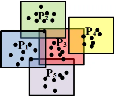
[image:9.595.209.414.367.535.2]D u (22d) After all the unique data samples are projected onto the DA planes, the next stage can start. Fig. 2 is an illustrative example of the DA planes that divide the whole data space while still being independent from each other, where the black dots stand for data samples, the blocks in different colours represent different DA planes in the data space. As one may also notice, some data samples are located in several DA planes at the same time, and their affiliations are decided by the distances between them and the origin points of the nearby DA planes.
Fig. 2 Illustrative example of the individual DA planes
3.3. Stage 3: Identifying the Focal Points
In this stage, for each DA plane, denoted as Pe , we consider the following rule, which find the
neighbouring DA planes, denoted by
n eP (l1, 2,..., ,L le):
Condition 2
, 2 , 2
M e l A e l
M A
n n
l
e e
d d
IF AND
d d
THEN
P P P
(23)
Let the corresponding D of
n eP be denoted by
n eD , if the following rule (Condition 3) is met, we
can claim that Pe stands for the main mode/peak of the data density.
Condition 3
e max
n
e /
e
IF D D THEN P is a mode peak of D (24)
By using Conditions 2 and 3 to examine each existing DA planes, one can find all the modes/peaks of the data density.
3.4. Stage 4: Forming Data Clouds
After all the DA planes standing for the modes/peaks of the data density are identified, we consider their origin points, denoted by
o , as the focal points and use them to form data clouds according to Condition 4(equation (25)) as a Voronoi tessellation [34]. It is worth to stress that the concept of data clouds is quite similar to the concept of clusters, but differs in the following aspects: i) data clouds are nonparametric; ii) data clouds do not have a specific shape; iii) data clouds represent the real data distribution.
Condition 4
1,2,..., , , arg min o oM l j A l j j C M A th l d d IF v d d
THEN is assigned to the v data cloud x x x (25)
where C is the number of the focal points.
3.5. SODA Data Partitioning Algorithm Summary
In this subsection, the main procedure of the proposed SODA partitioning algorithm is summarised in a form of pseudo code as follows.
SODA data partitioningalgorithm
i. Calculate dM and dAusing equations (17) and (18);
ii. Calculate the global density over the set
1, 2,...,
u
n
u u u using equation (16); iii. Rank
1, 2,...,
u
n
u u u based on their global density and obtain
ˆ ˆ1, 2,...,ˆ
u
n
u u u ;
iv. L1; v. 1uˆ1; vi. P1uˆ1; vii. S11; viii. 1 G
ˆ1n D
ix. While there are unassigned data samples in
ˆ ˆ2, 3,...,ˆ
u
n
u u u
1. IF (Condition 1 is met)
- Find the nearest DA plane using equation (20); - Update i,Si and Di using equations (21a)-(21c); 2. Else
- Create a new DA plane PL1;
- Update L,L,SL and DL using equations (22a)-(22d); 3. End If
x. End While
xi. Identify the neighbours of every existing DA plane using Condition 2;
xii. Identify the DA planes representing the modes/peaks using Condition 3;
xiii. Use the origin points of the identified DA planes as
o and form the data clouds using Condition 4.4. Extension of the
SODA
Algorithm for Processing Streaming Data
Many real problems and applications concern data streams rather than static datasets. In this section, an extension to the proposed SODA algorithm will be introduced to allow the algorithm to continue to process the streaming data on the basis of the partitioning results initiated by a static dataset. As a result, the main procedure of the SODA algorithm for streaming data processing will be built based on a structure initiated by an offline priming (does not start “from scratch”).
The main procedure of the SODA algorithm for the streaming data processing is as follows.
4.1. Stage 1: Meta-parameters Update
After the static dataset has been processed, for each newly arrived data sample from the data stream, denoted by xn1, nM ,
M n
X and nA are updated to 1 M n
, 1
M n
X and 1 A n
using equations (6), (7) and (9). The
values of the Euclidean components, dM and the angular components, dA between xn1 and the centres l ( 1, 2,...,
l L) of the existing DA planes are calculated using equations (1) and (2), denoted as dM
xn1,
l
and
1,
A n l
d x
, l1, 2,...,L.corresponding meta-parameters i,Si will be updated using equation (21a) and (21b). Otherwise, a DA plane
1 L
P is set up by xn1 and we update L,L,SL using equations (22a)-(22c).
4.2. Stage 2: Merging Overlapping DA Planes
After the Stage 1 is finished, Condition 5 is checked to identify the heavily overlapping DA planes in the data space ( ,i j1, 2,...,L,1 i j L):
Condition 5
, 1 , 1
2 2
M i j A i j
M A
i j
d d
IF AND
d d
THEN and are heavily overlapping
P P
(26)
If Pi and Pj( ,i j1, 2,...,L, 1 i j L) meet condition 5, we merge them together to create a new DA plane on the basis of Pj using the following principle:
1
L L (27a)
j i
j j i
j i j i
S S
S S S S
(27b)
j j i
S S S (27c)
Meanwhile, the meta-parameters of Pi are deleted. The merging process repeats until all the heavily overlapping DA planes have been merged. Then, the algorithm goes back to Stage 1 and waits for the newly coming data sample. If there is no new data sample anymore, the algorithm goes to the final stage.
4.3. Stage 3: Forming Data Clouds
Once there are no new data samples available, the SODA algorithm will quickly identify the focal points from the centres of the existing DA planes.
Firstly, the global densities of the centres l (l1, 2,...,L) of the DA planes are calculated using equation (16), where the support Sl (l1, 2,...,L) of each DA plane is used as the corresponding number of repeats. Here, the obtained global density is denoted as: DnG
l (l1, 2,...,L).Secondly, for each existing DA plane, Pe, Condition 2 (equation (23)) is used to find the neighbouring
DA planes around it, denoted as
n eP . Condition 3 (equation (24)) is used to check whether DnG
e is one ofthe local maxima of G
n lFinally, for all the identified local maxima of G
n lD
(l1, 2,...,L), the centres of the corresponding DA planes, denoted as
o , will serve as the focal points to form the data clouds using Condition 4.4.4. Algorithm Summary
In this subsection, we summarise and present the main procedure of the proposed SODA partitioning algorithm for streaming data processing in a form of pseudo-code as follows.
SODA partitioningalgorithm extension for streaming data processing
i. Start with the SODA algorithm for a priming data set and then
ii. While the new data sample xn is available 1. Update nM1 and XnM1 to nM and
M n
X using equations (6) and (7);
2. Calculate dM
xn,
l
and dA
x xi, j
using equations (1) and (2) 3. If (Condition 1 is met)- Find the nearest DA plane using equation (20); - Update i,Si and Di using equations (21a)-(21c); 4. Else
- Create a new DA planePL1;
- Update L,L,SL and DL using equations (22a)-(22d); 5. End If
6. IF (Condition 5 is met)
- Merge Pi and Pj using equations (27a)-(27c); - Remove the meta-parameters of Pi ;
7. End If
iii. End While
iv. Calculate G
n lD
(l1, 2,...,L) using equation (16);v. Identify the neighbours of every existing DA plane using Condition 2;
vi. Identify the DA planes representing the modes/peaks using Condition 3;
vii. Obtain the focal points
o ;5. Numerical Examples for the Proof of Concept
In this section, we will evaluate the performance of the proposed SODA partitioning algorithm on various challenging benchmark clustering problems and compare it with the performance of a number of “state-of-art” clustering algorithms. All the algorithms were implemented within MATLAB 2017a; the performance was evaluated on an ASUS laptop with dual i3 core processor with clock frequency 2.3GHz each and 8 GB RAM.
The following benchmark datasets are used in the experiments, where the abbreviations of the datasets used in the tables of this paper are also given:
i) S1 dataset [23];
ii) S2 dataset [23];
iii) Dim1024 dataset (D1024) [24];
iv) Dim15 dataset (D15) [29];
v) Fisher iris dataset (FI) [22];
vi) Wine dataset (WI) [1];
vii) Steel plate faults dataset (SP) [12];
viii) Occupancy detection dataset (OD) [14], where we removed the time stamps;
ix) Pen-based recognition of handwritten digits dataset (PB) [2].
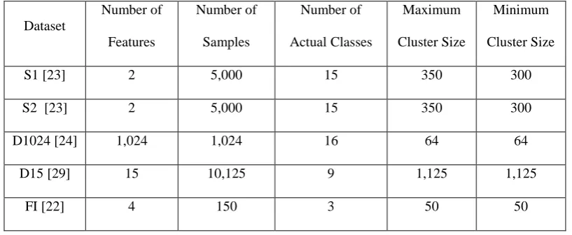
The details of the datasets are tabulated in Table I.
For different applications, one may also consider to rescale the value range of the data into
0,1 or [image:14.595.94.503.593.761.2]standardise the data with and
to make the majority located in the range of
3,3
as pre-processing, which may simplify the problems and improve the performance of the SODA data partitioning approach. Without loss of generality, in this paper, no pre-processing technique is used.Table I. Datasets used for evaluation
Dataset
Number of Features
Number of Samples
Number of Actual Classes
Maximum Cluster Size
Minimum Cluster Size
S1 [23] 2 5,000 15 350 300
S2 [23] 2 5,000 15 350 300
D1024 [24] 1,024 1,024 16 64 64
D15 [29] 15 10,125 9 1,125 1,125
WI [1] 13 178 3 71 48
ST [12] 27 1,941 7 673 55
OD [14] 5 20,560 2 15,810 4,750
PB [2] 16 10,992 10 1,144 1,055
5.1. Evaluation of the SODA Partitioning Algorithm and the Streaming Data Processing Extension
In this subsection, we will demonstrate the performance of the proposed SODA partitioning algorithm. For visual clarity, we only present the results of the S1, S2, D15 and OD datasets in Fig. 3, where the dots in different colours denote different data clouds. For D15 and OD datasets, which have more than 3 dimensions, we present the 3D partitioning results of the first 3 attributes. As one can see from Fig. 3, the proposed SODA algorithm successfully partitions the data samples based on their ensemble properties and groups similar data samples together.
(a) S1 dataset (b) S2 dataset
Fig.3. Partitioning results
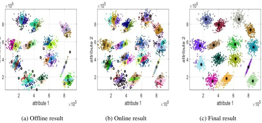
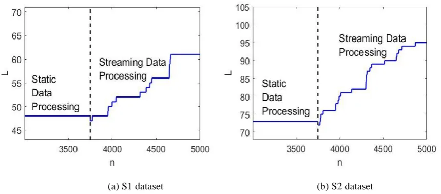
[image:16.595.83.502.278.474.2]The S1 and S2 datasets are further used to demonstrate the performance of the streaming data processing version of the SODA partitioning algorithm. In the following examples, 75% of the total data samples of two datasets are used as a static priming dataset for the SODA algorithm to generate the initial partitioning results. The rest of the data samples are transformed into data streams for the algorithm to continue to build upon the priming results. The overall results are presented in Figs. 4 and 5 where the black circle, “o” denotes the origin of the coordinates of the existing DA planes and the black asterisk, “*” represents the focal points extracted from the origins of the DA planes. The change of the number of direction-aware (DA) planes is also depicted in Fig. 6.
[image:16.595.80.503.506.701.2](a) Offline result (b) Online result (c) Final result Fig. 4 The streaming data processing version of the SODA algorithm (S1 dataset)
(a) S1 dataset (b) S2 dataset
Fig. 6. The evolution of the number of the DA planes during the processing of the data stream As we can see from Figs. 4(a) and 5(a), with the 75% of the data samples of the two datasets being processed statically, a number of DA planes are set up initially. Based on this initial result, the streaming data processing version can continue to assign the rest of the data samples and form data clouds when needed. With the arrival of new data samples, new DA planes will be set up along with the originally existing DA planes due to the dynamically evolving data pattern, see Fig. 4(b), 5(b). Once, there are no new data samples available, the focal points are identified by the SODA algorithm and the data clouds are formed around them, see Fig. 4(c) and 5(c). Thus, one can see that, using the results of the static datasets processing as a priming, the extension of the SODA algorithm can continue to process the streaming data in a “one-pass” mode. In contrast, the traditional offline clustering approaches lacks such ability and have to conduct clustering operation again based on all the previously observed data samples.
5.2. Comparison and Discussion
In this subsection, we will analyse and compare the performance of the proposed SODA partitioning algorithm versus the following “state-of-art” algorithms, where the short abbreviations of the algorithms used also in the tables of this paper are given as:
i) Subtractive clustering algorithm (SUB) [15];
ii) DBScan clustering algorithm (DBS) [21];
iii) Random swap algorithm (RS) [25];
iv) Message passing clustering algorithm (MP) [26];
v) Mixture model clustering algorithm (MM) [10];
vii) Evolving local means clustering algorithm (ELM) [20];
viii) Clustering of evolving data streams algorithm (CEDS) [28].
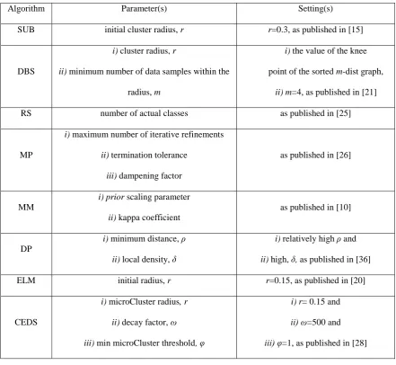
[image:18.595.77.519.207.613.2]In the experiments, due to the very limited prior knowledge, the settings of the free parameters of the comparative algorithms are based on the recommendations from the published literature. The experimental setting of the free parameters of the algorithms are presented in Table II.
Table II. Experimental Setting of the Algorithms
Algorithm Parameter(s) Setting(s)
SUB initial cluster radius, r r=0.3, as published in [15]
DBS
i) cluster radius, r
ii) minimum number of data samples within the
radius, m
i) the value of the knee
point of the sorted m-dist graph, ii) m=4, as published in [21]
RS number of actual classes as published in [25]
MP
i) maximum number of iterative refinements
ii) termination tolerance
iii) dampening factor
as published in [26]
MM
i) prior scaling parameter
ii) kappa coefficient
as published in [10]
DP
i) minimum distance, ρ
ii) local density, δ
i) relatively high ρ and
ii) high, δ, as published in [36]
ELM initial radius, r r=0.15, as published in [20]
CEDS
i) microCluster radius, r
ii) decay factor, ω
iii) min microCluster threshold, φ
i) r= 0.15 and
ii) ω=500 and
iii) φ=1, as published in [28]
For a better comparison, we consider the following quality measures to evaluate the clustering results: i) Number of clusters (C). Ideally, C should be as close as possible to the number of actual classes (ground
visual clarity and one can see that data samples from different classes have no obvious boundaries). The best way to cluster/partition the dataset of this type is to divide the data into smaller parts (i.e. more than one cluster per class) to achieve a better separation. At the same time, having too many clusters per class is also reducing the generalization capability (leading to overfitting) and the interpretability. Therefore, in this paper, we consider that the reasonable value range of C as number of actual classesC0.1number of samples. If C is smaller than the number of actual classes in the dataset or is more than 10% of all data samples, the clustering result is considered as an invalid one. The former case indicates that there are too many clusters generated by the clustering algorithm, which makes the information too trivial for users, and the latter case indicates that the clustering algorithm fails to separate the data samples from different classes.
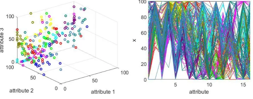
[image:19.595.76.498.293.459.2](a) 3D visualization of the first 3 attributes (b) 2D visualization of all the attributes
Fig. 7. Visualization of the Pen-based recognition of handwritten digits dataset (dots and lines in different colour represent data samples of different classes)
ii) Purity (P) [20], which is calculated based on the result and the ground truth:
1 N
i D i
S P
K
(28) where SDi is the number of data samples with the dominant class label in the ith cluster. Purity directly indicates separation ability of the clustering algorithm. The higher purity a clustering result has, the stronger separation ability the clustering algorithm exhibits.iii) Calinski-Harabasz index (CH) [13], the higher the Calinski-Harabasz index is, the better the clustering
result is;
iv) Davies-Bouldin index (DB) [17], the lower Davies-Bouldin index is, the better the clustering result is.
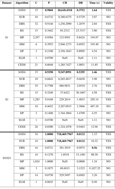
The comparison results using the datasets in Table I are tabulated in Table III. Table III. Performance comparison
Dataset Algorithm C P CH DB Time (s) Validity
S1
SODA 15 0.9860 20,618.4318 0.3752 1.64 YES
SUB 10 0.6732 8,360.6375 0.5729 3.07 NO
DBS 32 0.9146 1,256.2090 1.2679 2.84 YES
RS 15 0.3462 85.2312 23.3317 3.80 YES
MP 2,297 0.9584 123.9501 0.8424 194.97 NO
MM 6 0.3952 2,966.1273 0.6952 345.40 NO
DP 3 0.2100 2,356.1843 0.8905 4.54 NO
ELM 1 0.0700 NaN NaN 1.11 NO
CEDS 21 0.6048 1,285.7427 1.0851 11.85 YES
S2
SODA 15 0.9290 9,547.8991 0.5295 1.46 YES
SUB 10 0.6642 6,265.4817 0.6630 2.90 NO
DBS 35 0.7788 686.9831 2.0510 2.76 YES
RS 15 0.3240 37.6422 30.1067 4.58 YES
MP 1,283 0.9168 229.2614 1.4833 205.14 YES
MM 10 0.4652 2,207.0915 2.3866 407.10 NO
DP 2 0.1400 1,764.3864 1.4709 4.55 NO
ELM 1 0.0700 NaN NaN 1.11 NO
CEDS 26 0.6580 1,324.1078 0.9463 12.96 YES
D1024
SODA 16 1.0000 718,469.7967 0.0132 1.15 YES
SUB 16 1.0000 718,469.7967 0.0132 16.32 YES
DBS 16 0.8721 381.3919 0.9975 0.56 YES
RS 16 0.1270 1.0518 15.1481 88.30 YES
MP 1,024 1.0000 NaN 0.0000 1.34 NO
MM 3 0.1875 69.6915 3.1523 11,827.25 NO
DP 14 0.8750 529.5497 0.6965 3.26 NO
CEDS 8 0.5000 139.4129 1.4281 52.41 NO
D15
SODA 9 1.0000 302,436.3684 0.1177 2.99 YES
SUB 9 1.0000 302,436.3684 0.1177 25.15 YES
DBS 9 0.9586 20,602.057 1.2317 15.92 YES
RS 9 0.2455 129.4692 9.3269 10.28 YES
MP System Crashed NO
MM 4 0.4444 2,412.1759 1.4420 649.05 NO
DP 4 0.4444 4,533.2627 0.6696 13.65 NO
ELM 2 0.2222 3,319.7039 0.6205 2.58 NO
CEDS 76 0.6126 289.8403 2.2719 874.35 NO
FI
SODA 4 0.9533 398.2076 0.7570 0.38 YES
SUB 9 0.9533 288.7665 1.1278 0.21 YES
DBS 2 0.6600 226.6532 3.0295 0.15 NO
RS 3 0.7200 42.0557 2.2776 0.90 YES
MP 5 0.9133 440.6378 0.9267 0.34 YES
MM 1 0.3333 NaN NaN 6.50 NO
DP 2 0.6667 501.9249 0.3836 2.43 NO
ELM 1 0.3333 NaN NaN 0.17 NO
CEDS 16 0.6667 168.2046 1.5277 0.24 YES
WI
SODA 9 0.6966 400.2223 1.2734 0.83 YES
SUB 178 1.0000 NaN 0.0000 1.76 NO
DBS 4 0.6685 139.8891 1.9340 0.03 YES
RS 3 0.4775 0.5575 36.6770 1.06 YES
MP 51 0.8090 45.9785 0.5056 0.56 NO
MM 1 0.3988 NaN NaN 9.50 NO
DP 3 0.6461 321.3938 0.4782 2.49 YES
ELM 54 0.9719 7.6683 0.6812 0.70 NO
CEDS 178 1.0000 NaN 0.0000 0.08 NO
SUB 4 0.3988 494.1967 0.9100 4.37 NO
DBS 18 0.4858 57.8279 1.7112 0.51 YES
RS 7 0.4096 1.1539 24.1123 3.28 YES
MP 1,477 0.8563 6.9878 0.4486 33.37 NO
MM 2 0.3472 21.9988 0.1474 96.48 NO
DP 3 0.3478 1,224.2338 0.4226 2.40 NO
ELM 7 0.3730 84.1426 1.2951 2.88 YES
CEDS 2 0.3467 2.0546 18.6821 17.73 NO
OD
SODA 25 0.9762 8,993.6575 0.6526 4.81 YES
SUB 9 0.9498 19,878.6811 1.1872 30.81 YES
DBS 208 0.8514 134.4039 1.4789 190.85 YES
RS 2 0.7690 638.5256 3.6008 5.69 YES
MP System Crashed NO
MM 3 0.7691 4,420.7364 0.5037 1,062.11 YES
DP 2 0.7690 5,495.9202 0.5548 30.49 YES
ELM 1 0.7689 NaN NaN 3.18 NO
CEDS 13 0.8484 1,555.1093 3.3988 42.22 YES
PB
SODA 131 0.9006 510.4931 1.3721 9.05 YES
SUB 187 0.8454 382.6055 1.9995 100.09 YES
DBS 38 0.6209 312.9177 1.4997 16.11 YES
RS 10 0.1143 1.0495 75.16 13.30 YES
MP System Crashed NO
MM 41 0.9325 1,010.81 2.2504 3,727.38 YES
DP 7 0.5993 2,559.6071 1.3044 17.32 NO
ELM 9 0.3092 634.1555 2.1794 20.67 NO
CEDS 1 0.1041 NaN NaN 2,466.47 NO
Analysing the results shown in Table III, we can compare the proposed algorithm with the other clustering algorithms listed above as follows.
The proposed SODA algorithm is one of the most accurate and efficient algorithms among the ones considered in the thorough comparison. Its partitioning results constantly exhibit very high quality in all 9 benchmark problems. In addition, the SODA algorithm is autonomous, parameter-free (there is no problem- or user- specific parameters involved) partitioning algorithm and it does not require prior knowledge and assumptions about the data distribution or pattern. The algorithm generates the results based entirely on the ensemble properties of the observed data. In addition, the computation efficiency of the SODA algorithm does not deteriorate with the increase of dimensionality as well as the size of the dataset.
2) Subtractive clustering algorithm [15]
It is very accurate if the data has a Gaussian distribution. However, for the datasets with non-Gaussian distribution, the performance of the subtractive clustering algorithm decreases significantly. Moreover, its computation efficiency is largely influenced by the size of the dataset. It is not very efficient in dealing with large-scale datasets.
3) DBScan clustering algorithm [21]
This algorithm is one of the fastest algorithms. However, similarly to the subtractive clustering algorithm, its computational efficiency decreases with the growing size of the dataset. In addition, with the given pre-defined free parameters, its performance is not very good.
4) Random swap algorithm [25]
It requires the number of actual classes in the dataset to be known in advance, which is often impractical in real cases. Its performance and efficiency is also not high compared with other algorithms.
5) Message passing clustering algorithm [26]
This algorithm produces very good results on small-scale and simple datasets. However, its performance on large and complex datasets is very limited. In addition, this algorithm consumes a much larger amount of computation resources compared with other algorithms used in the comparison. The system crashed after a few minutes if the number of data samples in the dataset exceeds a certain threshold.
6) Mixture model clustering algorithm [10]
It can produce good results on some datasets. However, its computation efficiency is very low. It is also not good in handling high dimensional datasets.
7) Density peak clustering algorithm [36]
different classes in many cases. In addition, with the growth of the number of data samples, the difficulty of deciding the input selection for the users is also increasing.
8) Evolving local means (ELM) clustering algorithm [20]
ELM [20] was introduced as a dynamically evolving extension of the mean-shift algorithm. It is highly efficient as an evolving algorithm. However, with the recommended setting of free parameters, it failed to separate the data from different classes in many problems considered in this paper.
9) Clustering of evolving data streams algorithm [28]
This algorithm was the recently introduced in [28] for streaming data processing. It is able to follow the evolving data pattern of the data stream and group the samples into arbitrary shaped clusters. Nonetheless, based on the recommended experimental settings, this algorithm only produces effective clustering results on datasets with simpler structures, and it often fails in complex ones.
6. Conclusion
In this paper, we proposed a new autonomous data partitioning algorithm, named “Self-Organised Direction Aware (SODA)”. The SODA partitioning algorithm takes both the traditional distance metric and the angular similarity into consideration, thus, takes advantages of the spatial and angular divergence at the same time. By employing the nonparametric EDA operators, the proposed SODA algorithm can extract the ensemble properties and disclose the mutual distribution of the data merely based on the empirically observed data samples. Moreover, a streaming data processing extension is also proposed for the SODA algorithm, which enables the algorithm to partition the data streams starting with a brief offline set of data and using the obtained partitioning result of the static dataset and continuing on a per data sample basis further. Numerical examples have demonstrated that the proposed algorithm is able to perform clustering autonomously with very high computation efficiency and produces high quality clustering results in various benchmark problems.
The proposed SODA algorithm takes one step further compared with the traditional clustering/partitioning algorithms by considering both spatial and angular divergence, therefore, it can exhibit good performance on large-scale and high-dimensional problems without user- and data- dependent parameters, which are of paramount importance for real applications, where prior knowledge are more often insufficient.
7. Acknowledgement
This work was partially supported by The Royal Society grant IE141329/2014 “Novel Machine Learning Paradigms to address Big Data Streams”.
Reference
[1] S. Aeberhard, D. Coomans, and O. de Vel, “Comparison of classifiers in high dimensional settings,” Dept. Math. Statist., James Cook Univ., North Queensland, Australia, Tech. Rep, 92-02,1992.
[2] F. Alimoglu and E. Alpaydin, “Methods of combining multiple classifiers based on different representations for penbased handwriting recognition,” in Proceedings of the Fifth Turkish Artificial Intelligence and Artificial Neural Networks Symposium, 1996.
[3] F. A. Allah, W. I. Grosky, and D. Aboutajdine, “Document clustering based on diffusion maps and a comparison of the k-means performances in various spaces,” in IEEE Symposium on Computers and Communications, 2008, pp. 579–584.
[4] P. Angelov, Autonomous learning systems: from data streams to knowledge in real time. John Wiley & Sons, Ltd., 2012.
[5] P. Angelov, “Outside the box: an alternative data analytics framework,” J. Autom. Mob. Robot. Intell. Syst., vol. 8, no. 2, pp. 53–59, 2014.
[6] P. Angelov, X. Gu, and D. Kangin, “Empirical data analytics,” Int. J. Intell. Syst., DOI 10.1002/int.21899, 2017.
[7] P. P. Angelov, X. Gu, and J. Principe, “A generalized methodology for data analysis,” under review, 2017.
[8] P. Angelov and R. Yager, “A new type of simplified fuzzy rule-based system,” Int. J. Gen. Syst., vol. 41, no. 2, pp. 163–185, 2011.
[9] C. M. Bishop, Pattern recognition. New York: Springer, 2006.
[10] D. M. Blei and M. I. Jordan, “Variational inference for Dirichlet process mixtures,” Bayesian Anal., vol. 1, no. 1 A, pp. 121–144, 2006.
[11] I. Bojic, T. Lipic, and V. Podobnik, “Bio-inspired clustering and data diffusion in machine social networks,” in Computational social networks, Springer London, 2012, pp. 51–79.
[13] T. Caliński and J. Harabasz, “A dendrite method for cluster analysis,” Commun. Stat. Methods, vol. 3, no. 1, pp. 1–27, 1974.
[14] L. M. Candanedo and V. Feldheim, “Accurate occupancy detection of an office room from light, temperature, humidity and CO2 measurements using statistical learning models,” Energy Build., vol. 112, pp. 28–39, 2016.
[15] S. L. Chiu, “Fuzzy model identification based on cluster estimation.,” Journal of Intelligent and Fuzzy Systems, vol. 2, no. 3. pp. 267–278, 1994.
[16] D. Comaniciu and P. Meer, “Mean shift: A robust approach toward feature space analysis,” IEEE Trans. Pattern Anal. Mach. Intell., vol. 24, no. 5, pp. 603–619, 2002.
[17] D. L. Davies and D. W. Bouldin, “A cluster separation measure,” IEEE Trans. Pattern Anal. Mach. Intell., vol. 2, pp. 224–227, 1979.
[18] D. Dovzan and I. Skrjanc, “Recursive clustering based on a Gustafson-Kessel algorithm,” Evol. Syst., vol. 2, no. 1, pp. 15–24, 2011.
[19] M. S. Dresselhaus, G. Dresselhaus, R. Saito, and A. Jorio, “Raman spectroscopy of carbon nanotubes,” Phys. Rep., vol. 409, no. 2, pp. 47–99, 2005.
[20] R. Dutta Baruah and P. Angelov, “Evolving local means method for clustering of streaming data,” IEEE Int. Conf. Fuzzy Syst., pp. 10–15, 2012.
[21] M. Ester, H. P. Kriegel, J. Sander, and X. Xu, “A density-based algorithm for discovering clusters in large spatial databases with noise,” in International Conference on Knowledge Discovery and Data Mining, 1996, pp. 226–231.
[22] R. A. Fisher, “The use of multiple measurements in taxonomic problems,” Ann. Eugen., vol. 7, no. 2, pp. 179–188, 1936.
[23] P. Franti and O. Virmajoki, “Iterative shrinking method for clustering problems,” Pattern Recognit., vol. 39, no. 5, pp. 761–775, 2006.
[24] P. Franti, O. Virmajoki, and V. Hautamaki, “Fast agglomerative clustering using a k-nearest neighbor graph,” IEEE Trans. Pattern Anal. Mach. Intell., vol. 28, no. 11, pp. 1875–1881, 2006.
[25] P. Franti, O. Virmajoki, and V. Hautamaki, “Probabilistic clustering by random swap algorithm,” in IEEE International Conference on Pattern Recognition, 2008, pp. 1–4.
[27] G. Gallego, C. Cuevas, R. Mohedano, and N. García, “On the mahalanobis distance classification criterion for multidimensional normal distributions,” IEEE Trans. Signal Process., vol. 61, no. 17, pp. 4387–4396, 2013.
[28] R. Hyde, P. Angelov, and A. R. MacKenzie, “Fully online clustering of evolving data streams into arbitrarily shaped clusters,” Inf. Sci. (Ny)., vol. 382–383, pp. 96–114, 2017.
[29] I. Karkkainen and P. Franti, “Gradual model generator for single-pass clustering,” Pattern Recognit., vol. 40, no. 3, pp. 784–795, 2007.
[30] T. Larrain, J. S. J. Bernhard, D. Mery, and K. W. Bowyer, “Face recognition using sparse fingerprint classification algorithm,” IEEE Trans. Inf. Forensics Secur., vol. 12, no. 7, pp. 1646–1657, 2017.
[31] J. Li, S. Ray, and B. G. Lindsay, “A nonparametric statistical approach to clustering via mode identification,” J. Mach. Learn. Res., vol. 8, no. 8, pp. 1687–1723, 2007.
[32] A. Mathur, “Data Mining of Aviation Data for Advancing Health Management,” AeroSense 2002, pp. 61–71, 2002.
[33] G. J. McLachlan, “Mahalanobis Distance,” Resonance, vol. 4, no. 6, pp. 20–26, 1999.
[34] A. Okabe, B. Boots, K. Sugihara, and S. N. Chiu, Spatial tessellations: concepts and applications of Voronoi diagrams, 2nd ed. Chichester, England: John Wiley & Sons., 1999.
[35] X. Peng, L. Wang, X. Wang, and Y. Qiao, “Bag of visual words and fusion methods for action recognition: Comprehensive study and good practice,” Comput. Vis. Image Underst., vol. 150, pp. 109– 125, 2015.
[36] A. Rodriguez and A. Laio, “Clustering by fast search and find of density peaks,” Science, vol. 344, no. 6191, pp. 1493–1496, 2014.
[37] J. G. Saw, M. C. K. Yang, and T. S. E. C. Mo, “Chebyshev inequality with estimated mean and variance,” Am. Stat., vol. 38, no. 2, pp. 130–132, 1984.
[38] M. Senoussaoui, P. Kenny, P. Dumouchel, and T. Stafylakis, “Efficient iterative mean shift based cosine dissimilarity for multi-recording speaker clustering,” IEEE Int. Conf. Acoust. Speech Signal Process., pp. 7712–7715, 2013.
[39] V. Setlur and M. C. Stone, “A linguistic approach to categorical color assignment for data visualization,” IEEE Trans. Vis. Comput. Graph., vol. 22, no. 1, pp. 698–707, 2016.
[41] P. Viswanath and V. Suresh Babu, “Rough-DBSCAN: A fast hybrid density based clustering method for large data sets,” Pattern Recognit. Lett., vol. 30, no. 16, pp. 1477–1488, 2009.
[42] C. Wang, S. Member, J. Lai, and D. Huang, “SVStream : A Support Vector Based Algorithm for Clustering Data Streams,” IEEE Trans. Knowl. Data Eng., vol. 25, no. 1, pp. 1410–1424, 2011.