Periodicity and Solution of Rational Recurrence Relation of Order Six

(1)

Periodicity and Solution of Rational Recurrence

Relation of Order Six

Tarek F. Ibrahim1,2

1_{Department of Mathematics, Faculty of Sciences and Arts (S. A.), King Khalid University, Abha, KSA} 2_{Department of Mathematics, Faculty of Science, Mansoura University, Mansoura, Egypt}

Email: [email protected]

Received April 27, 2012; revised May 27, 2012; accepted June 3, 2012

ABSTRACT

Difference equations or discrete dynamical systems is diverse field whose impact almost every branch of pure and applied mathematics. Every dynamical system a_n₁  f a

 

n determines a difference equation and vise versa. We obtain

in this paper the solution and periodicity of the following difference equation.



 



1 2 4 1 3

n n n n n n n

x  x x  x x x x  5 , (1)

0,1,

n  where the initial conditions x5,x4,x3,x2,x1 and x0 are arbitrary real numbers with x1,x3 and x5 not equal to be zero. On the other hand, we will study the local stability of the solutions of Equation (1). Moreover, we give graphically the behavior of some numerical examples for this difference equation with some initial conditions.

Keywords: Difference Equation; Solutions; Periodicity; Local Stability

1. Introduction

Difference equations or discrete dynamical systems is diverse field whose impact almost every branch of pure and applied mathematics. Every dynamical system



1

n n determines a difference equation and vise

versa. Recently, there has been great interest in studying difference equations. One of the reasons for this is a ne-cessity for some techniques whose can be used in inves-tigating equations arising in mathematical models de-cribing real life situations in population biology, eco-nomic, probability theory, genetics, psychology, ...etc. Difference equations usually describe the evolution of certain phenomenta over the course of time. Recently there are a lot of interest in studying the global attractiv-ity, boundedness character the periodic nature, and giv-ing the solution of nonlinear difference equations. Re-cently there has been a lot of interest in studying the boundedness character and the periodic nature of nonlin-ear difference equations. Difference equations have been studied in various branches of mathematics for a long time. First results in qualitative theory of such systems were obtained by Poincaré and Perron in the end of nine-teenth and the beginning of twentieth centuries. For some results in this area, see for example [1-13].



a  f a

Although difference equations are sometimes very simple in their forms, they are extremely difficult to

un-derstand throughly the behavior of their solutions. Many researchers have investigated the behavior of the solution of difference equations for examples.

Cinar [1,2] investigated the solutions of the following difference equations









1 2 1

n n n n n n

x  x x x   x x2

(2)



 



1 2 4 1 3

n n n n n n n

x  x x x  x x x  5 , (1)

0,1,

n  where the initial conditions x5, x4, x3, 2,

x x1, and x0 are arbitrary real numbers with x1, 3

x and x5 not equal to be zero. On the other hand, we will study the local stability of the solutions of Equa-tion (1). Moreover, we give graphically the behavior of some numerical examples for this difference equation with some initial conditions.

Here, we recall some notations and results which will be useful in our investigation.

Let I be some interval of real numbers and Let 1

: k

F I  

0

I

, be a continuously differentiable function. Then for every set of initial conditions xk,x k1,

x I, the difference equation





1 , 1, , , 0,1,

n n n n k

x F x x  x n , (2)

has a unique solution

 

x_{n n k}_ [11].

Definition (1.1) A point x I is called an

equilib-rium point of Equation (2) if



, , ,



.

xF x x  x

That is, x_nx for , is a solution of Equation (2), or equivalently,

0

n

x is a fixed point of F.

Definition (1.2) The difference Equation (2) is said to

be persistence if there exist numbers m and M with 0 < m

≤M < ∞ such that for any initial x__k,x_{ }_k₁, , x₀



0,



there exists a positive integer N which depends on the initial conditions such that m≤xn≤M for all n≥N.

Definition (1.3) (Stability)

Let I be some interval of real numbers.

1) The equilibrium point x of Equation (2) is locally stable if for every ε > 0, there exists δ > 0 such that for

1 0

, , ,

k k

x x   x I with

1 0 ,

k k

x  x x    x  x  x 

we have x0 x  for all n≥−k.

2) The equilibrium point x of Equation (2) is locally asymptotically stable if x is locally stable solution of Equation (2) and there exists γ > 0, such that for all

1 0

, , ,

k k

x x   x I with

1 0 ,

k k

x  x x    x  x  x 

we have limnxnx.

3) The equilibrium point x of Equation (2) is global attractor if for all xk,x k₁, , x₀I, we have

limnxnx.

4) The equilibrium point x of Equation (2) is glob-ally asymptoticglob-ally stable if x is locally stable, and x

is also a global attractor of Equation (2).

5) The equilibrium point x of Equation (2) is unsta-ble if x not locally stable.

The linearized equation of Equation (2) about the

equi-librium x is the linear difference equation



 







1 0 , , , k n n

i i n i

y_ F x x x x_ y_





  

Theorem (1.4) [10] Assume that (real num-

bers) and

,

p q



0,1,2,



k  Then 1

p q 

is a sufficient condition for the asymptotic stability of the difference equation

1 0, 0,1, .

n n n k

x_ px qx_  n 

Remark (1.5) Theorem (1.4) can be easily extended to

a general linear equations of the form

1 1 0, 0,1,

n k n k k n

x p x     p x  n 

where p p1, 2, , pk (real numbers) and k



1,2



.

Then Equation (4) is asymptotically stable provided that

1 1 k i i p  



.

Definition (1.6) (Periodicity)

A sequence

 

x_{n n k}_

n

is said to be periodic with pe-riod p if xn p x for all n≥−k.

2. Solution and Periodicity

In this section we give a specific form of the solutions of the difference Equation (1).

Theorem (2.1)

Let

 

x_{n n k}_ be a solution of Equation (1). Then Equation (1) have all solutions and the solutions are



 



14 5 14 4 14 3 14 2

14 1 14 14 1

14 2 14 3 14 4 14 5

14 6 14 7 14 8

, , , ,

, , ,

1 , 1 , 1 , 1 ,

1 , 1 ,

n n n n

n n n

n n n n

n n n

x k x h x L x

x x x h Lk

x k x h x L x

x x x Lk h

                                    

where x5k x, 4h x, 3L x, 2,x1,x0.

Proof:

For n = 0 the result holds. Now suppose that n > 0 and that our assumption holds for n− 1. We shall show that the result holds for n. By using our assumption for n− 1, we have the following:



 



14 19 14 18 14 17 14 16 14 15 14 14 14 13

14 12 14 11 14 10 14 9

14 8 14 7 14 6

, , , ,

, , ,

1 , 1 , 1 , 1

1 , 1 ,

n n n n

n n n

n n n n

n n n

x k x h x L x

x x x h Lk

x k x h x L x

x x x Lk h

                                     

Now, it follows from Equation (1) that







      

14 5 14 6 14 8 14 10 14 7 14 9 14 11

1 1 1 1 1

n n n n n n n

x x x x x x x

Lk h L l h k

    

 



14 2 14

14 1 14 2

14 3 14 4 14 5

14 6 14 7 14 8

, ,

, 1 ,

1 , 1 , 1 ,

1 , 1 , .

n n

n n n

x x

x h Lk x k

x h x L x

x x x Lk

     h                        

Thus, the proof is completed.

Theorem (2.2)

Suppose that be a solution of Equation (1). Then all solutions of Equation (1) are periodic with pe-riod fourteen.

 

xn n k

 

Proof:

From Equation (1), we see that



 





 





 





 



1 2 4 1 3 5

2 1 1 3 2 4 5

3 2 2 1 1 3 4

4 3 1 1 2 2 3

5 2 6 1 7

8 1 9 2 5 10 4

11

1 1 1

1 & 1 & 1

1 & 1 &

n n n n n n n

n n n n n n n n

n n n n n n n n

n n n n n n n n

n n n n n n

n n n n n n n

n

x x x x x x x

x x x x x x x x

x x x x x x

x x x x x x x

x x                                                      

 n₃&xn₁₂xn₂&xn₁₃xn₁&xn₁₄xn

which completes the proof.

3. Stability of Solutions

In this section we study the local stability of the solutions of Equation (1).

Lemma (3.1)

Equation (1) have two equilibrium points which are 0 and 1.

Proof:

For the equilibrium points of Equation (1), we can write





x  x x x x x x  Then _x4__x3_,_i.e_. _x4__x3_₀

Thus the equilibrium points of Equation (1) is are 0 and 1.

Theorem (3.2)

The equilibrium points x0 and x1 are unstable.

Proof:

We will prove the theorem at the equilibrium point 1

x and the proof at the equilibrium point x0 by the same way.

Let be a continuous function de-fined by







6 : 0, 0,

f   



1, , , , ,2 3 4 5 6

 

1 3 5

 

2 4 6



f u u u u u u  u u u u u u

Therefore it follows that



 



1 3 5 2 4 6

f u u u u u u

  





 











2

2 1 3 5 4 6 2 4

2 1 3 5 2 4 6 0

. 6

f u u u u u u u u u

u u u u u u

     



 



3 1 5 2 4 6

f u u u u u u

  







2



4 1 3 5 2 4 6

f u u u u u u u

   



 



5 1 3 2 4 6

f u u u u u u

  







2



6 1 3 5 2 4 6

f u u u u u u u

   

At the equilibrium point x1 we have

1 1 1

f u p

    ,     f u₂ 1 p₂,

3 1 3

f u p

    ,     f u₄ 1 p₄,

5 1 5

f u p

    ,     f u₆ 1 p₆

Then the linearized equation of Equation (1) about 1

x is

1 1 2 1 3 2 4 3

5 4 6 5 0

n n n n

n n

y p y p y p y p y

p y p y

n              i.e.

1 1 2 3 4 5 0

n n n n n n n

y y y y y y y 

Whose characteristic equation is

6 5 4 3 2 _{1 0}

       

By the generalization of theorem (1.4) we have 1       1 1 1 1 1 1

which is impossible. This means that the equilibrium point x1 is unstable. Similarly, we can see that the equilibrium point x0 is unstable.

4. Numerical Examples

For confirming the results of this section, we consider numerical examples which represent different types of solutions to Equation (1).

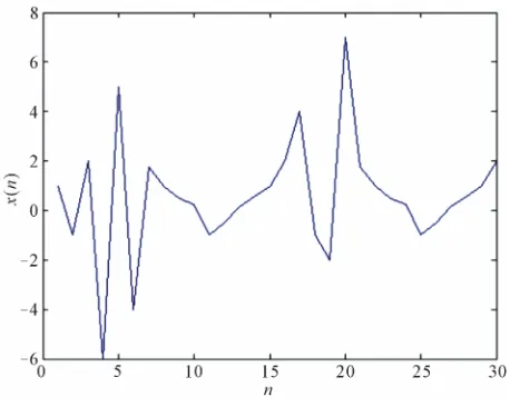
Example 4.1

Considerx−5 = 1, x−4 = 2, x−3 = 4, x−2 = −1, x−1 = −2, andx0 = 7. See Figure 1.

Example 4.2

Consider x−5 = 1, x−4 = −1, x−3 = 2, x−2 = −6, x−1 = 5, andx0 = −4. See Figure 2.

Example 4.3

Consider x−5 = 3, x−4 = 5, x−3 = −7, x−2 = −3, x−1 = 2, andx0 = −1. See Figure 3.



Example 4.4

(4)

[image:4.595.58.285.81.267.2] [image:4.595.309.536.83.262.2]

Figure 1. The periodicity of solutions with period 14 with unstable equilibrium points x = 1 and x = 0.

Figure 2. Periodicity of solutions with period 14 with unsta-ble equilibrium points x = 1, x = 0.

[image:4.595.58.287.309.492.2]

Figure 3. Periodicity of solutions with period 14 with unsta-ble equilibrium points x = 1 and x = 0.

Figure 4. The periodicity of solutions with period 14 with unstable equilibrium points x = 1, x = 0.

andx0 = −6. See Figure 4.

5. Acknowledgements

We want to thank the referee for his useful suggestions.

REFERENCES

[1] C. Cinar, “On the Positive Solutions of the Difference Equation xn1xn1



 1 ax xn n1



,” Applied

Mathemat-ics and Computation, Vol. 158, No. 3, 2004, pp. 793-797. doi:10.1016/j.amc.2003.08.139

[2] C. Cinar, “On the Positive Solutions of the Difference Equation xn1axn1



1bx xn n1



,” Applied

Mathemat-ics and Computation, Vol. 156, No. 2, 2004, pp. 587-590. doi:10.1016/j.amc.2003.08.010

[3] S. N. Elaydi, “An Introduction to Difference Equations,” Springer-Verlag Inc., New York, 1996.

[4] R. Karatas, C. Cinar and D. Simsek, “On Positive Solutions of the Difference Equation xn1xn5



1x xn2 n5



,”

In-ternational Journal of Contemporary Mathematical Sci-ences, Vol. 1, No. 10, 2006, pp. 495-500.

[5] T. F. Ibrahim, “On the Third Order Rational Difference Equation 1



2





1



x xn n2



,”

Interna-tional Journal of Contemporary Mathematical Sciences, Vol. 4, No. 27, 2009, pp. 1321-1334.

n n n n

x  x x x  

[6] T. F. Ibrahim, “Global Asymptotic Stability of a Nonlin-ear Difference Equation with Constant Coefficients,” Mathematical Modelling and Applied Computing, Vol. 1, No. 1, 2009.

[7] T. F. Ibrahim, “Dynamics of a Rational Recursive Se-quence of Order Two,” International Journal of Mathe-matics and Computation, Vol. 5, No. D09, 2009, pp. 98- 105.

[image:4.595.67.461.329.723.2]

(5)

Solu-tions of a Rational Difference Equation,” Journal of Pure and Applied Mathematics: Advances and Applications, Vol. 2, No. 2, 2009, pp. 227-237.

[9] T. F. Ibrahim, “Periodicity and Analytic Solution of a Recursive Sequence with Numerical Examples,” Journal of Interdisciplinary Mathematics, Vol. 12, No. 5, 2009, pp. 701-708.

[10] V. L. Kocic and G. Ladas, “Global Behavior of Nonlinear Difference Equations of Higher Order with Applications,” Kluwer Academic Publishers, Dordrecht, 1993.

[11] M. R. S. Kulenovic and G. Ladas, “Dynamics of Second Order Rational Difference Equations with Open Problems and Conjectures,” Chapman & Hall/CRC Press, Boca

Raton, 2001. doi:10.1201/9781420035384

[12] G. Ladas and M. Kulenovic, “On Period Two Solutions of xn1



  xnxn1

 

A B xnCxn1



,” Journal of

Difference Equations and Applications, Vol. 6, 2000, pp. 641-646.

[13] D. Simsek, C. Cinar and I. Yalcinkaya, “On the Recursive Sequence xn1xn3



1xn1



,” International Journal of