Missing Data Imputation for Ordinal Data

Missing Data Imputation for Ordinal Data

Maryuri Quintero

University of Texas at Arlington 701 S. Nedderman Drive

Arlington, TX 76019

Aera LeBoulluec,

701 S. Nedderman Drive Arlington, TX 76019

ABSTRACT

The treatment of missing data has become a mandatory step for performing valid data analysis in most scientific research fields. In fact, researchers have found that dealing with missing data avoids misleading data analysis and improves the quality and power of the research results [1]. According to the authors in [2,3], the missing values in a data set could be missing completely at random (MCAR), missing at random (MAR), or missing not at random (MNAR), a categorization that should be taken into consideration to deal with the problem of missing data. The number of observations, the types of variables, and the percentage of missing values in a data set are also important characteristics that should be contemplated before dealing with missing values. Understanding the missing data case helps the researchers to identify the imputation techniques that best handles the missing data problem. However, the development of procedures to impute categorical data is not significantly available as the procedures focused on continuous data imputation [1]. This study compares six different imputation methods to find the one that performs the most appropriate treatment for categorical data, type ordinal, in a breast cancer dataset.

General Terms

Data imputation; missing data.

Keywords

MCAR; categorical data; ordinal data.

1.

INTRODUCTION

The adequate analysis of data in all kinds of research fields is often hindered by the presence of missing information, a widespread problem that many data analysts face commonly. The occurrence of missing values arises from different reasons such as measurement errors, accidental deletion of recorded values, non-responses, and mistakes in data entry. As a result, analysts could end up drawing flawed conclusions about the data since the missing values have a detrimental effect when the data is analyzed [1]. In fact, some researchers argue that the performance of statistics on datasets with large amount of incomplete responses is significantly affected by the missing values [4]. According to the authors in [5], missingness in a dataset weakens the data analysis outcomes because the missingness brings ambiguity into the data analysis, reduces the statistical power of the data, and yields inaccurate statistical estimators such as means, variances, and percentages. The authors in [1,4] also support the idea that weak statistics, biased parameter estimates, loss of information, and inefficient standard errors result from the analysis of incomplete data. In brief, the missing values hold valuable information that is suppressed from the data analysis leading to erroneous findings.

Missingness can be appropriately handled through a variety of methods for imputing missing values. However, picking the right imputation method to treat the missing values depends

on the information known by the analyst such as the causes of missingness, the type of missingness in the dataset, and the type of data.

1.1

Types of Missing Values

The presence of missing observations is common in all kind of data collection, and this missingness could show different missing data patterns. Therefore, understanding the causes and patterns of missing data is crucial to perform a valid statistical analysis and select the best data treatment method. Rubin [2] considers that randomness behavior is the primary concern when the analyst deals with missing values. In fact, the author in [2] provides a basic classification of the types of missing data based on the randomness patterns that could emerge in a data due to problems in the data collection process.

The first type of missing data occurs when the data is missing completely at random (MCAR). This type of missing data happens when the cause of missingness in a variable has no relation with neither the missing values in that variable or the responses in other variables. Data missing completely at random usually results when a random subset of the study sample overlooks a question unintentionally leading to missingness in the data without a systematic cause. When data is MCAR, the missingness is under the control of the researcher, and the cause of missingness is some random event [6]. A good example of data MCAR occurs when some subjects of study neglected to answer a question in a survey because they did not see the question in the back of the survey form that they were filling out. Data MCAR could weaken the statistical power in the data, but this type of missingness does not cause significant bias in the data analysis outcomes because the respondents and nonrespondents do not share systematic differences [4].

the condition related to the missing values can be measured and used during the data analysis process.

Finally, data missing not at random (MNAR) is the third type of missingness that could emerge after the data collection process. This type of missingness occurs when the causes for missing values are unknown, and there is no way to get information about what is producing incomplete data. According to Finch [1], there is a high probability of getting data missing not at random in a variable when the responses are directly related to the value of the variable itself. For example, students who consume large amounts of cigarettes frequently are more likely to leave a question unanswered if they are asked to indicate the number of cigarettes they have consumed in the last week. This behavior results from the respondent’s need of hiding their real behavior leading to serious bias in the statistical analysis. In data MNAR, the missingness cannot be ignored as in data MAR, and the treatment of missing values become more difficult [4].

Unfortunately, when the data is missing systematically because of another variable (MAR or MNAR), the analyst could have a hard time trying to figure out the type of missing values, and making assumptions is the only way to determine these types of missingness and their influence on the data analysis [2,8]. In the case of MCAR, there is no correlation between the variable with missing values and another variable, so the information about the cause of missingness is not relevant in the data analysis to control the biases [6].

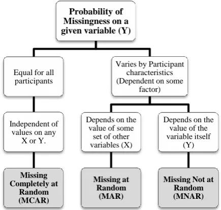
Classifying the types of missing values from the data is not an intuitively task, so Myers [9] presents a schema that simplifies the differences between the types of missing values and gives an approach to classify the missingness based on the probability of missingness on a given variable “Y” (see Figure 1).

Fig 1: Classification of the type of missing values based on the probability of missingness on a given variable “Y” [9]

1.2. Types of Data

The treatment of missing data requires methods that make appropriate assumptions for the type of data used in the study. So, identifying the type of data becomes a relevant step before conducting any action or analysis on the studied data. Quantitative data and qualitative data are the two basic types

of data that could be found in all kinds of research fields (see Figure 2).

Fig 2: Classification of the types of data

Quantitative data, also known as numerical data, results from numerical measurements that have meaningful values represented as a set of numbers. There are two different types of numerical data based on the scale of measurement for this type of data: discrete data and continuous data [10].

The first type of numerical data is discrete data, a type of data whose scale is made up of a list of possible numbers with gaps between them. The discrete data are only integer values (whole numbers) that can go to infinity or be part of a fixed list of numbers. According to the authors in [11], the discrete numbers can be counted, but they cannot be subdivided meaningfully because the data cannot be broken down into meaningful smaller units. Examples of discrete data are the number of defective parts in a production batch and the number of patients waiting for examination. Neither the defective parts nor the patients can be subdivided in significant smaller units. There is no such thing as “half of a defective part” or “one third of a patient”.

Continuous data is the second type of numerical data. Continuous data can take any numeric value in an interval because the measurement scale does not consider gaps between values measured. When the data is continuous, the numbers can be meaningfully subdivided into smaller parts (fractions and decimals), but the outcome values cannot be counted since there are infinite possible values that can result from the subdivision of a measured value. For instance, measurements of money, time, and temperature can be recorded and broken down into smaller parts, and the resulted numbers still have meaning. The time it takes an athlete to complete a race can be any value between a minimum and a maximum value of time, and this measure can be expressed in hours to fractions of a second.

Qualitative data, or categorical data, is the second basic type of data that could be found in research. The authors in [11] define categorical data as “data that can take on only a specific set of values representing a set of possible categories”. In similar words, categorical data are recorded observations placed into categories according to certain qualitative traits. This type of data cannot be numerically Probability of

Missingness on a given variable (Y)

Equal for all participants

Independent of values on any

X or Y.

Missing Completely at

Random (MCAR)

Varies by Participant characteristics (Dependent on some

factor)

Depends on the value of some

set of other variables (X)

Missing at Random

(MAR)

Depends on the value of the variable itself

(Y)

Missing Not at Random (MNAR)

Types of Data

Quantitative

(Numbers)

Continuous

(Fractions and decimales, no gaps

between values)

Discrete

(Integers, gaps between values)

Qualitative

(Categories)

Nominal

(Labels, No hierarchy)

Binary

(Two labels)

No Binary

(Multiple labels)

Ordinal

(Hierarchy)

Binary

(Two categories)

No Binary

measured like the numerical data type. The categorical data can be nominal, ordinal, or binary.

Nominal data is a type of qualitative data that falls into categories without any order or inherent ranking sequence. If the data is nominal, the values are represented with labels, words, letters or alphanumeric symbols that have no numerical significance. Gender and race categories are good examples of nominal data. When nominal data has two possible categories such as “Yes/No answers” or “female/male gender options”, the data is nominal and binary, and it is called dichotomous.

Categorical values can have a significant order or ranking. If the order of the data matters, the data is classified as ordinal data. Ordinal data can be counted and ordered, but it is not possible to measure it. In other words, the ordinal values are values assigned to hierarchical categories; the occurrences of observations per category can be counted, so there is mathematical meaning, but the value of the category is not meaningful mathematically if it is measured. For example, if 100 patients are asked to provide their level of satisfaction with their health insurance company by using a numerical scale from 1 (lowest) to 5 (highest), the outcome data will be the ordinal type, and the average of the 100 answers will have meaning. Ordinal data can have multiple categories, as shown in the example above, but binary ordinal data can happen if there are just two categories in a hierarchy.

The treatment of both numerical and categorical missing data has been studied for years in order to find the best imputation methods for different types of data. Since more approaches have been developed to deal with continuous data missingness [1], this study is focused on performing and comparing different imputation methods to find the one that best deals with ordinal data, a type of categorical data.

2.

DATA AND METHODOLOGY

2.1

Data Characteristics

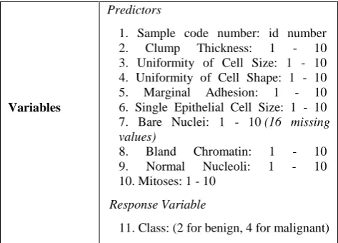
In the present study, a breast cancer dataset is used to perform and compare six different imputation methods. The dataset is a large multivariate dataset composed by 11 different variables and 699 observations whose values are integers resulted from an ordinal classification (see Table 1).

The breast cancer dataset was obtained from the University of Wisconsin Hospitals, and it was created by Dr. William H. Wolberg. This dataset can be found in the UCI Machine Learning Repository where there is available information about the data collection process and characteristics of the breast cancer database [12].

Table 1. Dataset information

Wisconsin Breast Cancer Dataset

Data

Characteristics Multivariate

Variable

Characteristics Integer

Type of Data Classification (Ordinal)

Number of

Observations 699

Number of

Variables 11 (10 predictors and 1 response variable)

Missing Values Yes. One predictor has 16 missing values.

Variables

Predictors

1. Sample code number: id number 2. Clump Thickness: 1 - 10 3. Uniformity of Cell Size: 1 - 10 4. Uniformity of Cell Shape: 1 - 10 5. Marginal Adhesion: 1 - 10 6. Single Epithelial Cell Size: 1 - 10 7. Bare Nuclei: 1 - 10 (16 missing values)

8. Bland Chromatin: 1 - 10 9. Normal Nucleoli: 1 - 10 10. Mitoses: 1 - 10

Response Variable

11. Class: (2 for benign, 4 for malignant)

2.2

Methodology

The breast cancer dataset includes ten (10) predictor variables of which just one has missing values. However, the variable with missing values was not included in this study in order to compare statistical measures in a complete dataset with the dataset imputed with different approaches. Then one variable with complete data, Uniformity of Cell Size, was selected to simulate different missing values levels. The variable

Uniformity of Cell Size has a high correlation with other variables in the dataset, which is convenient for performing better inferences in methods such as Multiple Imputation by Chained Equations that uses all the variables in a dataset to predict the missing values in the variable with missingness problems.

The missing values were introduced completely at random into the variable Uniformity of Cell Size leaving this variable with a percentage of missing values. One level of sample size (699 observed values) and seven levels of missing data were included in the variable of interest to analyze the performance of different imputation methods with varied percentage of missingness in the data.

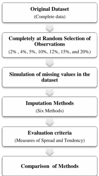
The first step to simulate the missing values was to get a completely-at-random sample of observations from the total observations recorded in the variable Uniformity of Cell Size. After obtaining a sub sample of values from the variable of interest, these values were replaced with empty responses to produce missingness in that variable. Seven levels of incomplete data Missing Completely at Random (MCAR) were simulated: 2%, 4%, 5%, 10%, 12%, 15%, and 20%. Then the simulated missing values were treated with six different imputation methods for each level of missing data included in the study. Finally, an evaluation criterion was used to measure the performance of all the imputation methods applied to the missing values for each level of missingness. The methodology used in this study is illustrated in the Figure 3.

Fig 3: Methodology used to compare different imputation methods in this study

The present study considers just those variables with complete data, so the measures performed on the imputed data can be compared with the measures made on the original complete data.

2.3

Evaluation criteria

Measures of spread and measures of central tendency were the parameters used as evaluation criteria in this study. The measures of spread are useful to analyze the similarity between the instances in the variable where missing values are imputed. Also, the measures of spread explain how scattered the observed values are in a dataset and how much these values differ from the mean value. On the other hand, the measures of central tendency produce a single value that describes all the values in the dataset and the central position within that set of data, which is useful to understand the data and its tendencies.

The variance and the standard deviation are the two measures of spread used for evaluating the different imputation methods in this study. Similarly, the mean value served as evaluation criteria to compare the central tendency between the imputed data and the original data (known values in the breast cancer database). These measures were calculated for both the original data and the imputed data for each imputation method and for each level of MCAR data involved in this study.

The percentage of error is a statistical tool that simplifies the comparison between experimental values and true values. Since the results of each imputation method aim for the original values in the data in this study, the calculation of the percentage of error was useful to determine the precision of each imputation method to predict the missing values in the variable of interest. The percentages of error closer to zero indicate that the imputation method produced values that were very close to the measures in the original dataset. The

Equation 1 is used to calculate the percentage of error in this study.

Where:

%Error = the percentage of error

Experimental value = the value obtained from the imputation method.

True value = the known data values.

The absolute difference between the experimental values and the true values is known as the absolute error, and it can be used as a simplified way to compare measures between the results of an experiment and the true values.

3.

IMPUTATION METHODS

Six different methods were used to treat the simulated missingness in the breast cancer dataset. A brief description of the assumptions for each imputation method is provided below.

3.1

The Most frequent value method

This method replaces the missing instances with the most common value within a set of values in a given variable. In other words, the method imputes the missing data with the number that is most likely to occur in a set of numbers in a variable.

3.2

Mean substitution method

The Mean Substitution method consists of replacing the missing data in a variable by the mean of all known values of that variable [5,13]. The mean is usually denoted by the symbol “ ”, and its value is equal to the sum of all the values in the variable divided by the total of observations in the variable. The mean calculation is represented in the Equation 2.

(2)

Where:

= the mean value

= the observations in the variable

= total number of observations

3.3

Random selection imputation

The Random Selection approach is a method based on randomly assigning a value to the missing data. The values randomly selected are framed in a specific range of values, which should have the same characteristics as the values in the variable with the missingness (numerical or categorical data). Each number in between the range has the same probability of being assigned to the missing data [14].

3.4

K-Nearest Neighbors classification

using Euclidean distance

The k-Nearest Neighbor method (KNN) is a conventional non-parametric classifier that uses the distances between the value treated and its k-nearest neighbors to find the final output for the value treated [5,15]. The KNN method defines a set of K nearest cases from the values treated and then estimates the replacement value from these neighbor cases selected [5]. The K-NN method uses the mean value to estimate the value for continuous data and the mode value to replace the missing values when the data is categorical [16]. Original Dataset

(Complete data)

Completely at Random Selection of Observations

(2% , 4%, 5%, 10%, 12%, 15%, and 20%)

Simulation of missing values in the dataset

Imputation Methods

(Six Methods)

Evaluation criteria

(Measures of Spread and Tendency)

One of the most common functions used for calculating the distance metrics in KNN is the Euclidean distance function. This function helps to measure the distances between two data points of interest in a feature space. The authors in [15] argue that, to calculate the distance between A and B, the normalized Euclidean metric can be determined by using the following equation:

₍₃₎

Let represent A and B by feature vectors A = (x1, x2,…, xm) and B = (y1, y2,…, ym), where m is the dimensionality of the feature space.

3.5

Multiple imputation by chained

equations

The authors in [5] define Multiple Imputation by Chained Equations (MICE) as “an iterative algorithm based on chained equations that uses an imputation model specified separately for each variable and involving the other variables as predictors” (p.1). In other words, MICE is a method that produces multiple predictions for the missing values by considering all the variables in the dataset as predictors. This method takes into consideration the statistical uncertainty when data is imputed by addressing the missingness problem with multiple imputations and a flexible approach to handle variables of different types of data [17]. The authors in [17] mention that when the MICE method is used, each variable with missing values is conditionally modeled based on the other variables in the data and uses its own distribution when repeated interactions between variables are performed. The iterations through all the variables are repeated until the process converges and a final complete dataset results from the imputed values.

3.6

Soft-Impute: Matrix completion by

iterative soft-thresholding of SVD

decompositions

Soft-Impute is an algorithm that iteratively replaces the missing values with values generated from a soft-thresholded SVD (Singular Value Decomposition). The Soft-Impute method facilitates the efficient regularization of solutions by computing a low-rank SVD of a dense matrix [18]. The Soft-Impute method uses parameters that consider low dimensionality, and when this method is performed, the values of the objective function decrease with each iteration producing minimum values in the function. This method repeatedly replaces the missing values with the current estimate, and then updates the estimate by solving an algorithm.

4.

RESULTS

Three main steps were performed to compare the six different imputation methods involved in this study: the calculation of evaluation metrics, the calculation of absolute errors, and the ranking of best imputation methods.

The calculation of evaluation metrics is the first step to compare the imputation methods included in this study. The mean value, the standard deviation, and the variance are the metrics defined as the evaluation criteria in this research, and they were calculated after performing each imputation method for different levels of missing values. The results from the calculation of the evaluation metrics for each imputation approach are provided in the Table 2. These same metrics were calculated for the original data before simulating missing values and applying any imputation approach. A mean equal to 3.134, a standard deviation equal to 3.051, and a variance equal to 9.0 are the values for the measures calculated in the original dataset. These measures are required to determine the following steps in this section.

The estimation of the absolute errors for each imputation method is the second step for the comparison of the imputation approaches included in this study. The calculation of the absolute errors was necessary to determine how well each imputation method performed in comparison to the original dataset characteristics. As it was mentioned in the section 3.3, the absolute errors result from the absolute difference between experimental values and true values. In this study, the absolute difference between the metrics of each imputation method and the metrics of the original data determines the absolute errors required in this research. For instance, if the evaluation metric is the standard deviation, the standard deviation of each imputation method is compared with the standard deviation of the original data. The absolute difference between those standard deviations estimates the absolute error for the studied case (see Equation 3).

An example of the absolute error calculation for the Multiple Imputation method (MICE) when the data has 2% of missing values and the evaluation metric is the standard deviation is as follow:

(3)

The absolute error for the MICE method when there is 2% of missing data and the evaluation metric is the standard deviation resulted equal to 0.047. This value shows how similar is the standard deviation of the MICE method to the standard deviation calculated for the original data under the given conditions. The same calculation was performed for each imputation method and for each evaluation metric under different missing data levels, which is summarized in the Table 3. In brief, the absolute error technique helped to identify how close were the imputed values from the original values in the breast cancer dataset.

Table 2. Evaluation criteria results after performing different imputation methods for different percentages of missingness

Table 3. Absolute errors between the evaluation criteria values of the original data and the imputed data for different percentages of missingness

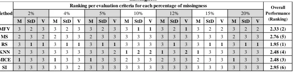
Table 4. Ranking of best imputation methods per overall performance and evaluation criteria for different percentages of missingness

The imputation method with a value equal to one (1) in an evaluation metric is the method with the best approach based on that criteria in a specific missingness level. The method with a criteria value equal to two (2) have the second place as a good method to approach the respective missingness case, and the methods with a criteria value equal to three (3) represent the ones that were least precise to predict the missing values. A ranking of the best imputation methods is shown in the Table 4, in which the best imputation methods are the ones with an overall performance closest to one (perfect performance level).

The Random Selection method (RS) was the imputation method with the best performance in this study. This method obtained the lowest percentage of errors for the standard deviations and variances in the majority of the missing levels cases except for 10% level of missingness, in which the method performed less precise than other methods. The Most

Frequent Value method (MFV) got the second place in the ranking of the best imputation methods because it generated the second most precise values in the evaluation criteria for all the missing values levels. The Multiple Imputation by Chained Equation method (MICE) and the K-Nearest Neighbor method (KNN) performed similarly in this study and achieved the following third and fourth places in the ranking of best imputation methods. The Mean Substitution method (MS) and the Soft-Impute method (SI) were the imputation techniques with the poorest performances in this study (see Table 4).

5.

CONCLUSION

In the present study, six imputation methods were performed to treat different missing values levels in a categorical dataset. These levels of missing values were simulated and introduced in a breast cancer dataset by following a completely at random

M StD V M StD V M StD V M StD V M StD V M StD V M StD V

MFV 3.087 3.018 9.111 3.052 3.011 9.069 3.031 3.004 9.022 2.914 2.950 8.700 2.877 2.931 8.592 2.798 2.911 8.474 2.715 2.855 8.152

MS 3.127 3.004 9.022 3.132 2.982 8.894 3.132 2.967 8.805 3.114 2.880 8.293 3.117 2.848 8.112 3.099 2.811 7.903 3.116 2.724 7.418

RS 3.170 3.054 9.000 3.237 3.070 9.000 3.282 3.085 9.000 3.454 3.177 10.000 3.461 3.166 10.000 3.489 3.158 9.000 3.578 3.121 9.000

KNN 3.127 3.017 9.100 3.130 3.010 9.059 3.127 2.997 8.979 3.133 2.937 8.626 3.134 2.916 8.501 3.136 2.884 8.318 3.206 2.801 7.846

MICE 3.130 3.004 9.025 3.133 2.983 8.898 3.136 2.968 8.808 3.132 2.883 8.312 3.127 2.850 8.123 3.117 2.816 7.929 3.139 2.728 7.441

SI 3.112 3.008 9.048 3.099 2.991 8.946 3.094 2.977 8.862 3.039 2.901 8.415 3.013 2.877 8.279 2.963 2.846 8.102 2.937 2.770 7.672

KNN = K-Nearest Neighbors MICE = Multiple Imputation by Chained Equations

SI = SoftImpute

Imputation Methods:

MFV = The Most Frequent Value MS = Mean Substitution RS = Random Selection

Evaluation Criteria:

M = Mean

StD = Standard Deviation V = Variance

Evaluation criteria values for the original data (before imputation)

M = 3.134 StD = 3.051 V = 9.000

2% 4% 5% 10% 12% 15% 20%

Method

Evaluation criteria results per percentage of missingness

M StD V M StD V M StD V M StD V M StD V M StD V M StD V

MFV 0.047 0.033 0.111 0.083 0.040 0.069 0.103 0.048 0.022 0.220 0.102 0.300 0.258 0.120 0.408 0.336 0.141 0.526 0.419 0.196 0.848

MS 0.007 0.048 0.022 0.003 0.069 0.106 0.003 0.084 0.195 0.020 0.172 0.707 0.017 0.203 0.888 0.036 0.240 1.097 0.019 0.328 1.582

RS 0.036 0.003 0.000 0.103 0.019 0.000 0.147 0.034 0.000 0.319 0.126 1.000 0.326 0.114 1.000 0.355 0.107 0.000 0.443 0.070 0.000

KNN 0.007 0.035 0.100 0.004 0.042 0.059 0.007 0.055 0.021 0.001 0.115 0.374 0.000 0.136 0.499 0.001 0.167 0.682 0.072 0.250 1.154

MICE 0.004 0.047 0.025 0.001 0.069 0.102 0.001 0.084 0.192 0.003 0.168 0.688 0.007 0.201 0.877 0.017 0.236 1.071 0.004 0.324 1.559

SI 0.023 0.044 0.048 0.036 0.061 0.054 0.040 0.075 0.138 0.096 0.151 0.585 0.122 0.174 0.721 0.172 0.205 0.898 0.197 0.282 1.328 Method

Absolute error per evaluation criteria and percentage of missingness

2% 4% 5% 10% 12% 15% 20%

M StD V M StD V M StD V M StD V M StD V M StD V M StD V

MFV 3 2 3 3 2 3 3 2 3 3 1 1 3 2 1 3 2 2 3 2 2 2.33 (2)

MS 2 3 2 2 3 3 2 3 3 3 3 3 3 3 3 3 3 3 2 3 3 2.76 (5)

RS 3 1 1 3 1 1 3 1 1 3 3 3 3 1 3 3 1 1 3 1 1 1.95 (1)

KNN 2 3 3 3 3 3 3 3 2 1 2 2 1 3 2 1 3 3 3 3 3 2.48 (4)

MICE 1 3 3 1 3 3 1 3 3 2 3 3 2 3 3 2 3 3 1 3 3 2.48 (3)

SI 3 3 3 3 3 2 3 3 3 3 3 3 3 3 3 3 3 3 3 3 3 2.95 (6)

20%

Overall Performance: The lowest value represents the imputation method with a better approach to treat the missingness in the breast cancer dataset.

Method

Ranking per evaluation criteria for each percentage of missingness _Overall

Performance (Ranking)

assumption. Then the performances of the six imputation methods were compared based on three evaluation criteria (Mean Value, Standard Deviation, and Variance).

The results show that the Random Selection method is the method with the best performance to treat the type of categorical data in this study (see Table 4). This method provided a small percentage of error when comparing the metrics for the imputed data with the metrics calculated for the original data. Other methods such as the Most Frequent Value, Multiple Imputation by Chained Equations, and the K-Nearest Neighbor Method offer secondary approaches to treat the data in this study.

In addition, the results in the current study demonstrate that the most commonly used imputation methods such as Mean and Multiple Imputation are not necessarily the most appropriate methods to treat categorical data, type ordinal. In fact, these methods achieved low positions in the ranking of the best methods for imputing the missing data case studied.

Performing the imputation methods used in this study to treat other types of categorical data, such as nominal data and binary categorical data, could serve as a supplementary research to evaluate the performance of these imputation methods under different scenarios. Moreover, further research can be performed to find appropriate approaches to treat categorical data that has other types of missingness patterns, such as MAR and MNAR.

The presence of missing data is a common problem that affects the data analysis process in all kinds of research projects. Although some researchers have studied and provided approaches for the treatment of missing values, there are still few procedures to impute the missingness in categorical data in comparison to the methods available for imputing continuous data. There is no universal method to impute data, but the results of this study suggest that the Random Selection method provides a good approach to handle the missingness problem in ordinal data, a type of categorical data.

6.

REFERENCES

[1] Finch, W. 2010. “Imputation methods for missing categorical questionnaire data: A comparison of approaches”. Journal of Data Science, vol. 8(8), pp. 361-378.

[2] Rubin, D. 1976. “Inference and missing data”. Biometrika, vol. 63(3), pp. 581-592.

[3] Little, R. and Rubin, D. 2002. “Introduction” in Statistical Analysis with Missing Data, 2nd ed., John Wiley & Sons, Inc., pp. 3-23.

[4] de Leeuw, D. and Huisman, M. 2003. “Prevention and treatment of item nonresponse”. Journal of Official Statistics, vol. 19(2), pp. 153-176.

[5] Schmitt, P., Mandel, J., and Guedj, M. 2015. “A comparison of six methods for missing data imputation”. Journal of Biometrics & Biostatistics, vol. 6(1), pp. 1-6.

[6] Graham, J. W., Hofer, S. M., Donaldson, S. I., MacKinnon, D. P., and Schafer, J. L. 1997. “Analysis

with missing data in prevention research” in The science of prevention: methodological advances from alcohol and substance abuse research, vol. 1, pp. 325-366.

[7] van der Heijden, G. J., Donders, A. R., Stijnen, T., and Moons, K. G. 2006. “Imputation of missing values is superior to complete case analysis and the missing-indicator method in multivariable diagnostic research: a clinical example”. Journal of Clinical Epidemiology, vol. 59(10), pp. 1102-1109.

[8] Schafer, J. L. and Graham, J. W.2002. “Missing data: our view of the state of the art”. Psychological Methods, vol. 7(2), pp. 147-177.

[9] Myers, T. A. 2011. “Goodbye, listwise deletion: Presenting hot deck imputation as an easy and effective tool for handling missing data”. Communication Methods and Measures, vol. 5(4), pp. 297-310.

[10] Bhattacharyya, G. and Johnson, R. 2014. Statistics: Principles and Methods. 7th edition. John Wiley & Sons, Inc. [E-book] Available: Safari e-book.

[11] Bruce, P. and Bruce, A. 2017. Practical Statistics for Data Scientists. 1st edition. O’Reilly Media, Inc. [E-book] Available: Safari e-book.

[12] Wolberg, W. 1992. “Breast Cancer Wisconsin (Original) Data Set”. Internet:

https://archive.ics.uci.edu/ml/datasets/breast+cancer+wis consin+(original)

[13] Olinsky, A., Chen, S., and Harlow, L. 2003. The comparative efficacy of imputation methods for missing data in structural equation modeling. European Journal of Operational Research, vol.151(1), pp. 53-79.

[14] Shrive, F. M., Stuart, H., Quan, H., and Ghali, W. A. 2006. “Dealing with missing data in a multi-question depression scale: a comparison of imputation methods”. BMC medical research methodology, vol. 6(1), pp. 57.

[15] Hu, L., Huang, M., Ke, S., and Tsai, C. 2016. “The distance function effect on k-nearest neighbor classification for medical datasets”. SpringerPlus, vol. 5, pp.1-9.

[16] García-Laencina, P. J., Sancho-Gómez, J. L., Figueiras-Vidal, A. R., and Verleysen, M. 2009. “K nearest neighbors with mutual information for simultaneous classification and missing data imputation”. Neurocomputing, vol. 72(7-9), pp. 1483-1493.

[17] Azur, M. J., Stuart, E. A., Frangakis, C., and Leaf, P. J. 2011. “Multiple imputation by chained equations: what is it and how does it work?”. International journal of methods in psychiatric research, vol. 20(1), pp. 40-49.