Vinod Ashokan1∗, N. D. Drummond2, and K. N. Pathak1
1Centre for Advanced Study in Physics, Panjab University, Chandigarh 160014, India and 2
Department of Physics, Lancaster University, Lancaster LA1 4YB, United Kingdom
We calculate the ground-state energy, pair correlation function, static structure factor, and mo-mentum density of the one-dimensional electron fluid at high density using variational quantum Monte Carlo simulation. For an infinitely thin cylindrical wire the predicted correlation energy is found to fit nicely with a quadratic function of coupling parameter rs. The extracted exponent
α of the momentum density fork ∼kF is used to determine the Tomonaga-Luttinger parameter
Kρ as a function of rs in the high-density regime for the first time. We find that the simulated
static structure factor and pair correlation function for infinitely thin wires agree with our recent high-density theory [K. Morawetzet al., Phys. Rev. B97, 155147 (2018)].
PACS numbers: 71.10.Hf, 71.10.Pm, 73.63.Nm, 73.21.Hb
I. INTRODUCTION
The quasi-one-dimensional uniform electron fluid has received much attention due to its interesting and the-oretically challenging behavior and potential technolog-ical applications.1,2 The advancement of material fabri-cation technology has permitted the realization of quasi-one-dimensional systems in carbon nanotubes,3–6 semi-conducting nanowires,7,8 confined cold atomic gases,9–11 edge states in quantum Hall liquids,12–14and conducting molecules.15
In this work we focus on high-density one-dimensional (1D) electron gases, which are strongly correlated sys-tems at all densities. Gold nanowires are an example of such a system. Experimentally one can create quan-tum wires by self-assembly from gold vapor. The gold atoms arrange themselves naturally on a stepped silicon surface to form a linear atomic chain.16 The linear elec-tron density for such a system isn1D= 1/(2rsa?B), where n1D= 1.3×107cm−1, rs is the coupling parameter, and the effective Bohr radius isa?B= [(κSi+1)/2](m0/m?)aB, where aB = 0.529 ˚A, the silicon dielectric constant is κSi = 11.5, and m? is the effective mass. The coupling constant isrs= 0.52 form?= 0.45m0,17andrs= 0.7 for m? = 0.60m
0.17,18 Another realization of a high-density 1D electron gas can be achieved in zigzag carbon nan-otubes placed on a SrTiO3 substrate, which has a high dielectric constant.19–21 These approaches stand in con-trast to the traditional way of obtaining a strongly corre-lated regime by lowering the electron densityn(or, equiv-alently, by increasing the coupling parameterrs) of a two-or three-dimensional electron gas. The latter approach suffers from the problem of localization by disorder be-cause of random charges on the substrate. The advantage of the former approach is that the Coulomb potential is strongly screened and the interaction among electrons is less affected by disorder. Potential applications of 1D
∗Corresponding author Email: [email protected]
electron systems include future silicon nanowire junc-tionless field-effect transistor technology.19,22,23 In such systems many-body effects including electron-electron in-teractions play an extremely important role in electronic transport.
It may be noted that the transverse confinement of the electrons modifies the effective electron-electron interac-tion potential and hence also plays a role in determining the properties of 1D electron systems. The effects of dif-ferent models of confinement have been studied by com-paring theoretical plasmon dispersions with experimental results.24 It has been found that the harmonic model of confinement with the proper dielectric constant of the substrate and effective mass of the electron wire mate-rial provides the closest description of wires fabricated on substrates.
The effects of interactions in one-dimensional (1D) physics are radically different from those in higher-dimensional physics. The famous Landau conventional Fermi liquid theory25,26 is not applicable in 1D due to the fact that single-particle excitation energies and their inverse lifetimes are of the same order of magni-tude. Further, the strength of these excitations is van-ishingly small at low energies. Therefore the prospect of observing non-Fermi-liquid features has given a large impetus to both theoretical and experimental research on 1D materials. Electron-like quasiparticle excitations are distinctive attributes of higher-dimensional physics, whereas in 1D such individual excitations do not ex-ist. The interaction in 1D turns the excitations into collective excitations, which are analogous to density os-cillations (spin or electronic density). The theory de-scribing the physical properties of 1D interacting sys-tems (fermions, bosons, or spins) is the Tomonaga-Luttinger (TL) liquid.27–29 The reduced dimensionality qualitatively changes the role of interactions, leading to phenomena such as spin-charge separation,30 charge fractionalization,31and Wigner crystallization.32
parameters completely determine the low-energy physics of the TL liquid.33 In the absence of interactionsv
ρ and vσ reduce to the Fermi velocity,vF, and the TL param-eters are equal to unity. For fermions K > 1 corre-sponds to attractive interactions and K < 1 repulsive interactions.34 For spin-rotation invariant (Kσ= 1) sys-tems, all exponents can be expressed in terms of one pa-rameter,Kρ. The spin-sector Kσ 6= 1 is possible only if spin rotation invariance is broken. The salient properties of a TL liquid are33(i) a continuous momentum distribu-tion funcdistribu-tionn(k) varying as|k−kF|αaround the Fermi wavenumberkF, withαbeing the interaction-dependent exponent, and a pseudogap in the single-particle den-sity of states N(ω) that is proportional to |ω|α, which is a consequences of the absence of fermionic quasiparti-cles; (ii) correlation functions follow similar nonuniversal power laws, with interaction-dependent exponents; and (iii) spin-charge separation, with spin and charge degrees of freedom propagating at different velocities.
The exactly solvable TL liquid model describes elec-tron correlations with short-range interactions. How-ever, the electrons in a real 1D homogeneous electron gas (HEG) interact via a long-range Coulomb interac-tion. The long-range character of the Coulomb poten-tial has been studied by Schulz.35Further, the mapping of the long-range Coulomb interaction onto an exactly solvable model with short-range behavior has been stud-ied by Fogler.21,36 In spite of these works the effects of long-range behavior within the TL model are still not fully understood. The harmonically transversally con-fined wire with finite width b has been studied with a lattice-regularized diffusion Monte Carlo technique by Casula et al.,37 and by others.38–40 Several theoretical works have investigated the 1D HEG within Fermi liquid theory,41–52and have been compared with the simulation results of Casulaet al.37with limited success.
Recently, the ground-state properties of the 1D elec-tron liquid for an infinitely thin wire, and the harmonic wire have been studied using the quantum Monte Carlo (QMC) method by Lee and Drummond53 for coupling parameters rs ≥ 1. In the present work we study the ground-state properties of infinitely thin and transver-sally confined harmonic wires using QMC as imple-mented in thecasinocode54in the high-density regime, i.e.,rs<1. The realistic long-range Coulomb interaction is taken to be 1/|x|, as studied by Lee and Drummond.53 From the simulated momentum density (MD) we have extracted its exponentαaroundk∼kF, which allows us to find the TL parameter Kρ as a function of rs in the high-density regime for the first time. The TL parameter Kρ we obtain at high density smoothly goes over to the value we obtained for low density from the data of Lee and Drummond.53
It is found that variational quantum Monte Carlo (VMC) correlation energies vary quadratically with rs in the high-density limit. Further, the simulated static structure factor (SSF) and pair correlation function (PCF) for infinitely thin wires are found to agree with
our recent high-density theory.55
The paper is organized as follows. The theoretical models used in our calculations for infinitely thin and harmonic wires are described in Sec. II. In Sec. III we outline our computational methodology, and provide the details of our approach. In Sec. IV we present results and discussion pertaining to the ground-state properties of the 1D HEG at high density. Finally, our overall conclu-sions are drawn in Sec. V. In this article we use Hartree atomic units (~=|e|=me= 4π0= 1) throughout.
II. THEORETICAL MODEL
The Hamiltonian for an N-electron 1D HEG is53
ˆ H =−1
2 N X
i=1 ∂2 ∂x2
i
+X
i<j
V(xij) + N
2VMad, (1)
where V(xij) and VMad are the Ewald interaction and Madelung energy respectively. The Ewald interaction of an electron at xi with an electron at xj in an in-finitely thin wire, determined by using Euler-Maclaurin summation,56 is
V(xij) = ∞ X
n=−∞
1 |xij+nL|
− 1 L
Z L/2
−L/2
dy |xij+nL−y|
,(2)
and for the harmonically confined wire the Ewald-like interaction potential is53
V(xij) = ∞ X
m=−∞
π 2be
(xij−mL)2/(4b)2erfc
|xij−mL 2b
− 1
|xij−mL| erf
|x
ij−mL 2b
+2 L
∞ X
n=1
E1[(bGn)2] cos(Gnxij), (3)
where b is the width of the wire in units of the Bohr radius, G = 2π/L, and E1 is the exponential integral function. The Madelung constant VMad is the electro-static potential at one electron due to all its periodic images (excluding itself); e.g., for the infinitely thin wire the Madelung constant is
VMad= lim x→0
V(x)− 1 |x|
. (4)
III. COMPUTATIONAL METHOD
0 2
×10-4 4×10⁻⁴ 6×10⁻⁴ 8×10⁻⁴ N -2
-1×10⁻² -8×10⁻³ -6×10⁻³ -4×10⁻³ -2×10⁻³ 0
E - E
∞
(a.u. / elec.)
r s=0.7 r
s=0.6 r
s=0.5 r
s=0.4 r
s=0.3 r
s=0.2
FIG. 1: (Color online) VMC energy (E−E∞) plotted against
the reciprocal of the square of the system size for the infinitely thin wire. The energies per particle were extrapolated to the thermodynamic limit using the formE(N) =E∞+BN−2.
a ferromagnetic system, the orbitals in the Slater de-terminants were plane waves with wavenumbers k / kF = π/(2rs). Using a backflow transformation58 pro-vides an effective way to describe the three-body corre-lations in a 1D HEG. The free parameters in the trial wave function were optimized by unreweighted variance minimization,59–61and energy minimization.62The prop-erties of the Slater-Jastrow-backflow trial wave function have been discussed in detail in Ref. 53, where it has been concluded that for infinitely thin wires the curva-ture of the wave function does not cancel the divergence in the interaction potential; hence the trial wave function possesses nodes at all of the coalescence points (i.e., at both like↑↑and unlike↑↓spin pairs). For infinitely thin 1D wires the ground-state energy is independent of the spin polarization, i.e., paramagnetic and ferromagnetic states are degenerate, which implies the inapplicability of the Lieb-Mattis theorem,63 whereas the ground-state energy is dependent on density. In the case of the har-monic wire, the paramagnetic and ferromagnetic sates
are nondegenerate and there is nontrivial dependence on the spin polarizationζ=|N↑−N↓|/N. However, in this work we restrict ourselves to calculations for the fully spin-polarized (ζ= 1) ferromagnetic fluid.
We have performed our calculations using only VMC. This is due to the fact that the VMC and diffusion Monte Carlo (DMC) results differ insignificantly. For example, forrs≥1, Lee and Drummond53 found VMC to retrieve more than 99.999% of the correlation energy, while the VMC and extrapolated DMC estimates of the MD differ by no more than∼2 error bars.
IV. RESULT AND DISCUSSION
Ground-state energy: We have calculated VMC
ground-state energies for rs = 0.1, 0.2, 0.3, 0.4, 0.5, 0.6, 0.7, 0.8, and 0.9, with the number of electrons be-ingN = 37, 55, 77, and 99 for both infinitely thin and harmonic wires, and we have extrapolated to the ther-modynamic limit. These results are given in Table I. For infinitely thin wires the energies per particle were extrapolated to the thermodynamic limit using the form E(N) =E∞+BN−2, whereBandE∞are fitting param-eters, which was derived in Ref. 53 using the method pro-posed in Ref. 64. This form is also in agreement with con-formal field theory results.65,66 We used the same func-tional form for finite-size extrapolation of the energies of harmonic wires. Figure 1 shows that this form fits the energy per particle of an infinitely thin wire well, and allows extrapolation to the thermodynamic limit. We used a Slater-Jastrow-backflow wave function for both infinitely thin and finite-thickness systems at high den-sity, as used by Lee and Drummond53 for low-density calculations. For the infinitely thin wire withrs = 0.9, N = 99, and ζ = 1, the error bars on the ground-state energy were O(10−7) a.u. per electron. The correlation energies for infinitely thin and harmonic wires are calcu-lated from the VMC ground-state energy.
The exchange energy is obtained52as
x(rs, ζ) =− 1 8rs
(1 +ζ)2
3
2−γ+β−ln
π(1 +ζ) 4rs
+L
+ (1−ζ)2
3
2 −γ+β−ln
π(1−ζ) 4rs
+L
, (5)
where ζ is the spin polarization, γ is Euler’s constant andL =−ln(b). For infinitely thin wire β = 0 and for thin harmonic wireβ = (γ/2)−ln(2). Note that the logarithmic thickness of the wire is defined byL−1, and Lcancels with the neutralizing background in the thermodynamic limit.
In Fig. 2, the correlation energy is plotted againstrs, and it is fitted with the quadratic function c(rs) = −0.027431(3) + 0.00791(1) rs −0.00196(1) r2s, where the constant and coefficient are in agreement with the conventional perturbation theory result,67 i.e.,
c(rs) = −0.0274156 + 0.00845 rs+. . . for high densities. The
correlation energy for the harmonic wire of widthb= 0.5 in the high-density limit is fitted with a quadratic func-tion c(rs, b = 0.5) = 0.00079(1) −0.00581(4) rs − 0.00062(3) r2
[image:3.595.64.291.52.212.2]0 0.2 0.4 0.6 0.8 1
r
s
-0.028 -0.027 -0.026 -0.025 -0.024 -0.023 -0.022 -0.021
ε c
(a.u. / elec.)
VMC, b=0, ζ=1
VMC, b=0.5, ζ=1
0 0.2 0.4 0.6 0.8 1 -0.006
-0.005 -0.004 -0.003 -0.002 -0.001 0 0.001
FIG. 2: (Color online) Correlation energycas a function of
rs for an infinitely thin wire (and in the inset for a harmonic
[image:4.595.329.548.50.401.2]wire of width b= 0.5). The solid line is a quadratic fit as a function ofrs.
TABLE I: VMC ground-state total energiesE∞extrapolated
to the thermodynamic limit and correlation energiescfor the
infinitely thin wire (b= 0) and harmonic wire (b= 0.5).
Infinitely thin wire Harmonic wire
E∞ c E∞ c
rs
(a.u./elec.) (a.u./elec.) (a.u./elec.) (a.u./elec.) 0.1 50.25356(3) −0.026707(3) 40.31883(2) −0.00023(2) 0.2 13.10051(1) −0.025921(1) 9.52997(1) −0.00050(1) 0.3 5.765347(7) −0.025199(7) 3.861399(5) −0.000981(5) 0.4 3.102011(5) −0.024559(5) 1.898573(5) −0.001581(5) 0.5 1.842920(5) −0.023960(5) 1.004636(4) −0.002239(4) 0.6 1.151946(3) −0.023389(3) 0.529594(3) −0.002924(3) 0.7 0.734582(3) −0.022865(3) 0.251097(3) −0.003616(3) 0.8 0.465155(1) −0.022361(1) 0.076506(2) −0.004285(2) 0.9 0.2825597(9) −0.0218909(9) −0.038302(2) −0.004929(2)
data in Table I) becomes unphysically positive.
Pair correlation function: The parallel-spin PCF is defined as
g↑↑(x) = 1 ρ2
↑ N↑
X
i>j
δ(|xi,↑−xj,↑| −x)
, (6)
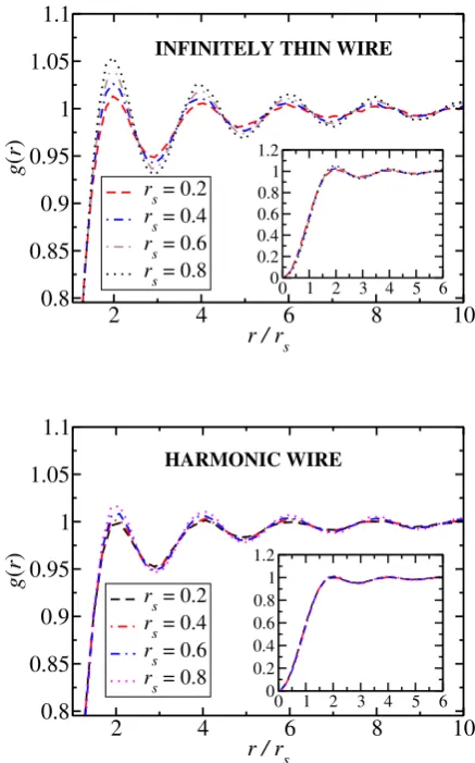
where ρσ is the electron density for spin σ, xi,↑ is the position of the ith electron with spin σ, and the angu-lar bracketsh· · · idenote an average over configurations distributed as the square modulus of the wave function. The PCFs for an infinitely thin wire and a harmonic wire of thickness b = 0.5 are plotted in Fig. 3 for sev-eral values of rs <1. In Fig. 4 we have compared the simulation with our recent high-density theory55 for in-finitely thin wires, which was obtained in theb→0 limit for cylindrical wires. It may be recalled that the random phase approximation is known to lead to negative values ofg(r) at small distances,55 and this artifact is removed
2 4 6 8 10
r / rs 0.8
0.85 0.9 0.95 1 1.05 1.1
g
(
r
)
rs = 0.2
rs = 0.4
rs = 0.6
rs = 0.8
0 1 2 3 4 5 6
0 0.2 0.4 0.6 0.8 1 1.2
INFINITELY THIN WIRE
2 4 6 8 10
r / rs 0.8
0.85 0.9 0.95 1 1.05 1.1
g
(
r
)
rs = 0.2
rs = 0.4
rs = 0.6
rs = 0.8
0 1 2 3 4 5 6
0 0.2 0.4 0.6 0.8 1 1.2
HARMONIC WIRE
FIG. 3: (Color online) (upper) PCF of an infinitely thin wire at several densities. (lower) PCF of a harmonic wire of width b= 0.5 at several densities. The data shown are forN = 99. The inset shows the same data at the origin. The random errors in the data are small, as evidenced by the lack of visible noise in the curves.
in the high-density theory which takes into account the vertex correction.
Static structure factor: The SSFS(k) is defined in terms of the PCF as
S(k) = 1 +N L
Z
[g(x)−1]e−ikxdx, (7)
whereg(x) isg↑↑(x) in this case. The SSF contains infor-mation about the phase of the system. By using Eq. (6) in Eq. (7) we obtain an expression forS(k) which shows that it is a measure of the average squared amplitude of density fluctuations of wavenumberk.
[image:4.595.72.285.51.205.2] [image:4.595.55.303.315.473.2]0
1
2
3
4
5
6
r
0
0.2
0.4
0.6
0.8
1
g
(
r
)
r s=0.2 r
s=0.4 r
s=0.6 r
s=0.8 r
s=0.9
0 1 2 3 4
0.92 0.96 1 1.04 1.08
Solid line (Theory)
INFINITELY THIN WIRE
FIG. 4: (Color online) PCFs g(r) of 1D HEGs in infinitely thin wires. Results obtained from VMC simulation are com-pared with recent high-density theory55 at several densities.
The inset shows the oscillations ofg(r) at larger distances in greater detail.
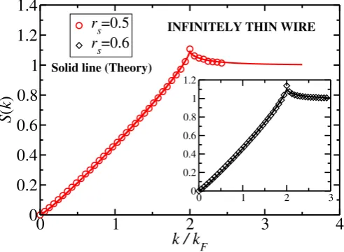
that the SSF as a function of the wavenumber shows the typical uncorrelated behavior at high density with the double Fermi wavenumber 2kF as characteristic inverse length. Also we have compared the simulation with the analytical expression for the SSF as given in the high-density theory.55As shown in Fig. 7, the theoretical SSF calculated from the formula (given in Appendix A for ready reference) and the simulated SSF are in excellent agreement.
1.9
2
2.1
2.2
k / k
F1
1.1
1.2
1.3
S
(
k
)
N
=99
N
=77
N
=55
N
=37
0 1 2 3 4
0 0.35 0.7 1.05 1.4
INFINITELY THIN WIRE
FIG. 5: (Color online) SSF of an infinitely thin wire at several system sizes forrs= 0.8. The main plot shows the behavior
at the peak and the inset shows a zoomed-out view.
In Fig. 6 we have plotted the SSF peak height at k = 2kF against N, and it is fitted with a function S(k = 2kF) = a+b/N. In the thermodynamic limit the peak height tends to a constant value. Forrs= 0.5, 0.6, 0.7, 0.8, and 0.9, the height becomes a = 1.12976, 1.14735, 1.17464, 1.22649, and 1.25001, respectively. As
30
40
50
60
70
80
90
100
N
1
1.1
1.2
1.3
1.4
1.5
S
(
k
=2
k
F) peak height
VMC, r
s=0.9
VMC, r
s=0.8
VMC, r
s=0.7
VMC, r
s=0.6
VMC, r
s=0.5
INFINITELY THIN WIRE
FIG. 6: (Color online) SSF peak height atk = 2kF plotted
against system sizeN for infinitely thin wires with different coupling parametersrs.
0
1
2
3
4
k / k
F
0
0.2
0.4
0.6
0.8
1
1.2
1.4
S
(
k
)
r
s=0.5
r
s
=0.6
0 1 2 3
0 0.2 0.4 0.6 0.8 1 1.2 Solid line (Theory)
INFINITELY THIN WIRE
FIG. 7: (Color online) VMC SSF of an infinitely thin wire withN= 99, compared with the high-density theory55(solid line). The main plot shows the SSF forrs= 0.5 and the inset
is forrs= 0.6.
we increase the coupling parameterrs, the peak height in the thermodynamic limit is also increased.
Momentum density: The MD is a fundamental
quantity and it is calculated from the ground-state trial wave function using the formula
n(k) = 1 2π
Z ψ
T(r) ψT(x1)
exp[ik(x1−r)]dr
, (8)
where the trial wave function, ψT(r) is evaluated at (r, x2, . . . , xN). The angular brackets denote the VMC expectation value, obtained as the mean over electron coordinates (x1, . . . , xN) distributed as|ψT|2.
[image:5.595.62.294.49.210.2] [image:5.595.322.553.50.220.2] [image:5.595.318.564.276.456.2] [image:5.595.54.300.417.595.2]0.8 0.9 1 1.1 1.2 k / k
F
0 0.2 0.4 0.6 0.8 1
n
(
k
)
r s = 0.9 r
s = 0.8 r
s = 0.7 r
s = 0.6 r
s = 0.5 r
s = 0.4 r
s = 0.3
0 0.5 1 1.5 2
0 0.2 0.4 0.6 0.8 1
INFINITELY THIN WIRE
0.8 0.9 1 1.1 1.2
k / k
F
0 0.2 0.4 0.6 0.8 1
n
(
k
)
r s = 0.9 r
s = 0.8 r
s = 0.7 r
s = 0.6 r
s = 0.5 r
s = 0.4 r
s = 0.3
0 0.5 1 1.5 2
0 0.2 0.4 0.6 0.8 1
HARMONIC WIRE
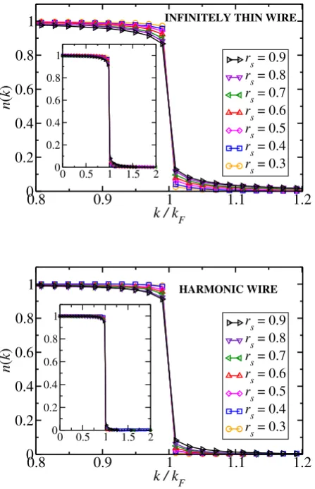
FIG. 8: (Color online) (upper) MD of an infinitely thin wire and (lower) MD of a harmonic wire of widthb= 0.5 at sev-eral densities. The data shown are forN = 99. The statistical error bars are much smaller than the symbols and have there-fore been omitted for clarity. The inset shows a zoomed-out view.
for a free-electron (noninteracting) system, and the spec-tral function for free electrons is a delta-function peak. Now when the interaction is switched on, the remarkable Landau Fermi liquid theory applies and the properties of the system remain essentially similar to those of free fermionic particles. The elementary particles are not the individual electrons anymore, but are dressed by the den-sity fluctuations around them and are called quasiparti-cles. The MDn(k) of a state with momentumkstill has a discontinuity at the Fermi wavenumberk=kF (the spec-tral function possesses a quasiparticle peak), but with reduced amplitude Z < 1. On the other hand, in 1D the interaction leads to a power-law behavior in the MD, which is continuous at kF, though the derivative of the MD is singular at k=kF. Near the Fermi wavenumber the TL liquid theory predicts the MD should take the form28,68
n(k) =n(kF) +A[sign(k−kF)]|k−kF|α (9)
where n(kF), A, and α are density-dependent
parame-ters. The exponentαmay be written in terms of the TL parameterKρ as69
α= 1 4
Kρ+
1 Kρ
−2
. (10)
0 0.05 0.1 0.15 0.2
Fitting range ε
0 0.04 0.08 0.12 0.16 0.2 0.24 0.28 0.32
Exponent
α
r s=0.9 r
s=0.8 r
s=0.7 r
s=0.6 r
s=0.5 r
s=0.4 r
s=0.3
INFINITELY THIN WIRE
0 0.05 0.1 0.15 0.2
Fitting range ε
0 0.04 0.08 0.12 0.16 0.2 0.24 0.28 0.32
Exponent
α
r
s=0.9
r s=0.8 r
s=0.7 r
s=0.6 r
s=0.5 r
s=0.4 r
s=0.3 HARMONIC WIRE
FIG. 9: (Color online) Tomonaga-Luttinger liquid exponentα in Eq. (9) extracted from our MDs against the fitting range of data (|k−kF|< kF), for (upper) a ferromagnetic, infinitely
thin wire and (lower) a harmonic wire of widthb= 0.5 The extracted exponent is linearly fitted with the solid line in the region >0.035 and extrapolated to= 0.
[image:6.595.66.290.50.397.2] [image:6.595.332.546.81.464.2]0.3 0.4 0.5 0.6 0.7 0.8 0.9
r
s 0
0.05 0.1 0.15 0.2
Exponent
α
b=0, ζ=1
b=0.5, ζ=1
FIG. 10: (Color online) Exponentα, found by fitting Eq. (9) to the MDs of ferromagnetic 1D electron gases and extrap-olating to = 0, plotted against rs. The error bars on the
data points approximately account for the random error due to the Monte Carlo evaluation of the momentum density of the trial wave function (approximate because the data points in the MD are correlated); however, the random noise on the exponents is clearly larger than these error bars. There is an additional uncertainty in the MD and hence α due the stochastic optimization of the trial wave function, and this may be responsible for the larger noise. Nevertheless, the noise in the exponentαas a function ofrsis at least an order
of magnitude smaller than the systematic behavior.
0
0.2
0.4
0.6
0.8
1
b
0.015
0.02
0.025
0.03
0.035
0.04
0.045
0.05
0.055
Exponent
α
VMC ζ=1 Cubic fit
HARMONIC WIRE
FIG. 11: (Color online) Exponentαfound by fitting Eq. (9) to the MDs of ferromagnetic systems forrs= 0.5 and different
harmonic wire widthsb.
Lee and Drummond53for lower density. The variation of the exponentαwithrs is plotted in Fig. 10. It is found that in the high-density limit α tends to zero, whereas Lee and Drummond53have found that in the low-density limit α tends to 1. The exponent α for rs = 0.5 as a function of the width b of the wire is shown in Fig. 11. As the width of the harmonic wire decreases the exponent αincreases. Using a cubic fit the exponent is extrapolated tob= 0, givingα= 0.0538(6), which agrees with the result for an infinitely thin wire [α= 0.0505(2) atrs= 0.5].
0
5
10
15
20
r
s0
0.2
0.4
0.6
0.8
1
K
ρVMC DMC Fitted
0 0.2 0.4 0.6 0.8 1 α
0 0.2 0.4 0.6 0.8 1
Kρ Analytical
INFINITELY THIN WIRE
FIG. 12: (Color online) Tomonaga-Luttinger parameterKρ
plotted againstrs and, in the inset, plotted as a function of
exponentαfor an infinitely thin wire. The low density DMC data are adopted from Lee and Drummond.53
Further, the TL parameter is obtained from Eq. (10) as Kρ = 1 + 2α−2
√
α+α2. It is noted that for re-pulsive interactions Kρ is positive and < 1. The value of α is approximately given by α = tanh(rs/8).53 This formula continues to describe the value ofα forrs < 1 for the infinitely thin wire, although the fractional error increases significantly whenrs≤0.5. When substituted in the relation betweenKρ andα, this yields
Kρ = 1 + 2 tanh(rs/8)
−2 q
tanh(rs/8) + tanh2(rs/8). (11)
This is plotted in Fig. 12 as function ofrs (and in the inset as a function ofα). The low-density data have been taken from Lee and Drummond.53The TL parameterK
ρ we obtain for high density smoothly goes over to the value we obtained for low density from the data of Lee and Drummond.53 The TL parameterK
ρis well represented by the formula given in Eq. (11) for the infinitely thin wire.
In the present work the TL liquid behavior is charac-terized by the power-law decay in the momentum dis-tribution function at the Fermi wavenumber. The TL parameter Kρ gives a quantitative value of the corre-lation strength. Small values of the TL parameter Kρ imply a strongly correlated system. The results in Fig. 12 immediately indicate non-Fermi liquid behavior. In other words, we confirm in the present study that how-soever small the interaction may be, the electron fluid in 1D behaves as a TL Liquid. We further observed that the structure factor at k = 2kF has a peak even in the high-density regime.
[image:7.595.71.282.50.205.2] [image:7.595.322.552.52.215.2] [image:7.595.58.295.369.530.2]1D electron fluid are not yet available.
V. CONCLUSIONS
We have performed a detailed VMC study of 1D elec-tron fluids interacting via long-range Coulomb potentials for infinitely thin and harmonic wires at high density. For the infinitely thin and harmonic-wire models, we have reported the VMC ground-state energy in the thermo-dynamic limit. Using the VMC ground-state energy we have calculated the correlation energy. The predicted correlation energy is in agreement with conventional per-turbation theory results67 at high densities. The calcu-lated SSF shows a peak at 2kF. The VMC SSF and PCF data show very good agreement with the high-density theory.55
Forrs<1 we have reported VMC results for the MD as function of wavenumberk, and the data are used to predict the Tomonaga-Luttinger parameter for infinitely thin and harmonic wires. It is found that the exponentα ranges from 0.02 to 0.12 in the high-density limit. The ex-ponent has been used to obtain the Tomonaga-Luttinger parameterKρ as a function of rs. It is hoped that our work will motivate experimental work on high-density 1D electron systems. One example of a suitable material for study is a zigzag carbon nanotube placed on a SrTiO3 substrate.
Acknowledgments
The authors (V.A. and K.N.P.) acknowledge the finan-cial support by National Academy of Sciences of India,
Allahabad. The high performance computing centre fa-cilities at Panjab University has been used to run the casinocode for our QMC calculations.
Appendix: A
The analytical expression for the SSF in the high-density theory55 forx <1 is
S(k) = x 2 +
g2 srs π2x
(x−2) ln 2−x
2
[ln(4−2x)
−2(ln(x) + 1)] + (x+ 2) ln x+ 2
2
×[2 ln(x)−ln(2x+ 4) + 2]
, (A.1)
wherex=k/kF, and forx >1
S(k) = 1 +g 2 srs π2x
(2−x) ln2(x−2)−(x+ 2) ln2(x+ 2)
+2(x−2)[ln(x) + 1] ln(x−2)−2xln(x)[ln(x) + 2]
+2(x+ 2)[ln(x) + 1] ln(x+ 2)
. (A.2)
The PCFg(r) is obtained from the SSFS(k) as
g(r) = 1− 1 2πn
Z ∞
−∞
dk eikr[1−S(k)]. (A.3)
1 G. F. Giuliani and G. Vignale, Quantum theory of the
electron liquid (Cambridge University Press, Cambridge, 2005).
2 T. Giamarchi, Quantum Physics in One Dimension
(Clarendon, Oxford, 2004).
3
R. Saito, G. Dresselhaus, and M. S. Dresselhaus,Physical Properties of Carbon Nanotubes (Imperial College Press, London, 1998).
4
M. Bockrath, D. H. Cobden, J. Lu, A. G. Rinzler, R. E. Smalley, L. Balents, and P. L. McEuen, Nature397, 598 (1999).
5
H. Ishii, H. Kataura, H. Shiozawa, H. Yoshioka, H. Ot-subo, Y. Takayama, T. Miyahara, S. Suzuki, Y. Achiba, M. Nakatake, T. Narimura, M. Higashiguchi, K. Shimada, H. Namatame, and M. Taniguchi, Nature426, 540 (2003).
6
M. Shiraishi and M. Ata, Sol. State Commun. 127, 215 (2003).
7
J. Sch¨afer, C. Blumenstein, S. Meyer, M. Wisniewski, and R. Claessen, Phys. Rev. Lett.101, 236802 (2008).
8 Y. Huang, X. Duan, Y. Cui, L. J. Lauhon, K.-H. Kim, and
C. M. Lieber, Science294, 1313 (2001).
9
H. Monien, M. Linn, and N. Elstner, Phys. Rev. A 58, R3395 (1998).
10 A. Recati, P. O. Fedichev, W. Zwerger, and P. Zoller, J.
Opt. B: Quantum Semiclass. Opt.5, S55 (2003).
11
H. Moritz, T. Stoferle, K. Guenter, M. Kohl, and T. Esslinger, Phys. Rev. Lett.94, 210401 (2005).
12
F. P. Milliken, C. P. Umbach, and R. A. Webb, Sol. State Commun.97, 309 (1996).
13 S. S. Mandal and J. K. Jain, Sol. State Commun.118, 503
(2001).
14
A. M. Chang, Rev. Mod. Phys.75, 1449 (2003).
15
A. Nitzan and M. A. Ratner, Science300, 1384 (2003).
16 T. Nagao, S. Yaginuma, T. Inaoka, and T. Sakurai, Phys.
Rev. Lett.97, 116802 (2006).
17
K. N. Altmann, J. N. Crain, A. Kirakosian, J.-L. Lin, D. Y. Petrovykh, F. J. Himpsel, and R. Losio, Phys. Rev. B 64, 035406 (2001).
18
R. Losio, K. N. Altmann, A. Kirakosian, J.-L. Lin, D. Y. Petrovykh, and F. J. Himpsel, Phys. Rev. Lett.86, 4632 (2001).
19
A. Javey, H. Kim, M. Brink, Q. Wang, A. Ural, J. Guo, P. McIntyre, P. McEuen, M. Lundstrom, and H. Dai, Nat. Mater.1, 241 (2002).
20
21
M. M. Fogler, Phys. Rev. B71, 161304 (2005).
22 J.-P. Colinge, C.-W. Lee, A. Afzalian, N. D. Akhavan, R.
Yan, I. Ferain, P. Razavi, B. O’Neill, A. Blake, M. White, A.-M. Kelleher, B. McCarthy, and R. Murphy, Nat. Nan-otechnol.5, 225 (2010).
23 M. M. Mirza, F. J. Schupp, J. A. Mol, D. A. MacLaren,
G. Andrew, D. Briggs, and D. J. Paul, Sci. Rep.7, 3004 (2017).
24 R. K. Moudgil, V. Garg, and K. N. Pathak, J. Phys.:
Con-dens. Matter22, 135003 (2010).
25
L. D. Landau, J. Exp. Theor. Phys.8, 70 (1958).
26 P. Nozieres, Theory of Interacting Fermi Systems
(Ben-jamin, New York, 1961).
27
S. Tomonaga, Prog. Theor. Phys.5, 544 (1950).
28 J. M. Luttinger, J. Math. Phys.4, 1154 (1963). 29
F. D. M. Haldane, Phys. Rev. Lett.47, 1840 (1981).
30
O. M. Auslaender, H. Steinberg, A. Yakoby, Y. Tserkovnyak, B. I. Halperin, K. W. Baldwin, L. N. Pfeiffer, and K. W. West, Science308, 88 (2005).
31
H. Steinberg, G. Barak, A. Yacoby, L. N. Pfeiffer, K. W. West, B. I. Halperin, and K. Le Hur, Nat. Phys. 4, 116 (2008).
32
V. V. Deshpande and M. Bockrath, Nat. Phys. 4, 314 (2008).
33 J. Voit, Rep. Prog. Phys.5897 (1995). 34
H. J. Schultz, G. Cuniberti, and P. Pieri,Field Theories for Low-Dimensional Condensed Matter System. G. Morandi et al.(Eds.), Springer (2000); preprint cond-mat/9807366.
35
H. J. Schulz, Phys. Rev. Lett.71, 1864 (1993).
36
M. M. Fogler, Phys. Rev. Lett.94, 056405 (2005).
37 M. Casula, S. Sorella, and G. Senatore, Phys. Rev. B74,
245427 (2006).
38
L. Shulenburger, M. Casula, G. Senatore, and R. M. Mar-tin, Phys. Rev. B78, 165303 (2008).
39 A. Malatesta and G. Senatore, J. Phys. IV10, 5 (2000). 40
A. Malatesta,Quantum Monte Carlo study of a model one-dimensional electron gas, (Ph.D thesis, Universita Degli studi Di Trieste, Departmento di Fisica Teorica) (1999).
41
S. Capponi, D. Poilblanc, and T. Giamarchi, Phys. Rev. B 61, 13410 (2000).
42 G. Fano, F. Ortolani, A. Parola, and L. Ziosi, Phys. Rev.
B60, 15654 (1999).
43
D. Poilblanc, S. Yunoki, S. Maekawa, and E. Dagotto, Phys. Rev. B56, R1645 (1997).
44 B. Valenzuela, S. Fratini, and D. Baeriswyl, Phys. Rev. B
68, 045112 (2003).
45 M. Fabrizio, A. O. Gogolin, and S. Scheidl, Phys. Rev.
Lett.72, 2235 (1994).
46
W. I. Friesen and B. Bergersen, J. Phys. C13, 6627 (1980).
47 L. Calmels, and A. Gold, Phys. Rev. B56, 1762 (1997). 48 V. Garg, R. K. Moudgil, K. Kumar, and P. K. Ahluwalia,
Phys. Rev. B78, 045406 (2008).
49
M. Ta¸s and M. Tomak, Phys. Rev. B67, 235314 (2003).
50 R. Bala, R. K. Moudgil, Sunita Srivastava and K. N.
Pathak, J. Phys.: Condens. Matter24245302 (2012).
51
R. Bala, R. K. Moudgil, Sunita Srivastava, and K. N. Pathak, Eur. Phys. J. B875 (2014).
52
V. Ashokan, R. Bala, K. Morawetz, and K. N. Pathak, Eur. Phys. J.91, 29 (2018).
53 R. M. Lee and N. D. Drummond, Phys. Rev. B83, 245114
(2011).
54
R. J. Needs, M. D. Towler, N. D. Drummond, and P. L´opez R´ıos, J. Phys. Condens. Matter22, 023201 (2010).
55 K. Morawetz, V. Ashokan, R. Bala, and K. N. Pathak,
Phys. Rev. B97, 155147 (2018).
56
V. R. Saunders, C. Freyria-Fava, R. Dovesi, and C. Roetti, Comp. Phys. Commun.84, 156 (1994).
57
N. D. Drummond, M. D. Towler, and R. J. Needs, Phys. Rev. B70, 235119 (2004).
58 P. L´opez R´ıos, A. Ma, N. D. Drummond, M. D. Towler,
and R. J. Needs, Phys. Rev. E74, 066701 (2006).
59
C. J. Umrigar, K. G.Wilson, and J. W. Wilkins, Phys. Rev. Lett.60, 1719 (1988).
60
P. R. C. Kent, R. J. Needs, and G. Rajagopal, Phys. Rev. B59, 12344 (1999).
61 N. D. Drummond and R. J. Needs, Phys. Rev. B 72,
085124 (2005).
62
C. J. Umrigar, J. Toulouse, C. Filippi, S. Sorella, and R. G. Hennig,Phys. Rev. Lett.98, 110201 (2007).
63 E. Lieb and D. Mattis, Phys. Rev.125, 164 (1962). 64
S. Chiesa, D. M. Ceperley, R. M. Martin, and M. Holz-mann, Phys. Rev. Lett.97, 076404 (2006).
65 I. Affleck, Phys. Rev. Lett.56, 746 (1986). 66
H. W. J. Bl¨ote, J. L. Cardy, and M. P. Nightingale, Phys. Rev. Lett.56, 742 (1986).
67 P. F. Loos, J. Chem. Phys.138, 064108 (2013). 68
D. C. Mattis and E. H. Lieb, J. Math. Phys.6, 304 (1965).
69