Determination of Full Energy Peak Efficiency of NaI(Tl)
Detector Depending on Efficiency Transfer Principle for
Conversion Form Experimental Values
Mohamed Abd-Elzaher1*, Mohamed Salem Badawi2, Ahmed El-Khatib2, Abouzeid Ahmed Thabet1
1Department of Basic and Applied Science, Faculty of Engineering, Arab Academy for Science,
Technology and Maritime Transport, Alexandria, Egypt
2Physics Department, Faculty of Science, Alexandria University, Alexandria, Egypt
Email: *[email protected]
Received March 18, 2012; revised April 22, 2012; accepted May 11,2012
ABSTRACT
In this work we calibrated the NaI(Tl) scintillation detectors (5.08 × 5.08 cm2 and 7.62 × 7.62 cm2) and the Full Energy
Peak Efficiency (FEPE) for these detectors have been calculated for point sources placed at different positions on the detector axis using the analytical approach of the effective solid angle ratio. This approach is based on the direct mathematical method reported by Selim and Abbas [1,2] and has been used successfully before to calibrate the cylin-drical, parallelepiped, and 4π NaI(Tl) detectors by using point, plane and volumetric sources. In addition, the present method is free of some major inconveniences of the conventional methods.
Keywords: Full Energy Peak Efficiency; NaI(Tl) Scintillation; Efficiency Transfer
1. Introduction
Determination of detector efficiency is very important in various scientific and industrial fields. Because the perimental work is tedious and even difficult for ex-tended sources, many researches have been focused on the development of computational techniques to deter-mine these efficiencies. There are three famous methods used in this field, the semi-empirical, the Monte Carlo, and the direct mathematical methods. One of these com-putational techniques is the efficiency transfer method in which the computation of the detector efficiency for various geometrical conditions is derived from the known efficiency for a reference source-detector geometry. The main advantage of the Efficiency Transfer approach with a point calibration source located at a sufficient distance from the detector is that one may neglect coincidence summing effects and obtain a coincidence free efficiency curve [3]. The efficiency transfer method is particularly useful due to its insensitivity to the inaccuracy of the input data, e.g. to the uncertainty of the detector charac-terization [4,5].
Change in efficiency under conditions of measurement different from those of calibration can be determined on the basis of variation of the geometrical parameters of the source-detector arrangement. By calculation, it is
possi-ble to determine the efficiency corresponding to non-point samples and/or different distances. The basic case corre-sponds to calibration with known efficiency for a point source located at position, Pο, at energy, E, the efficiency
can be expressed as:
E, Pο
i
E eff
Pο (1)
where, i
E , represents the intrinsic efficiency of the detector for energy, E, and, Ωeff(Po), is the solid anglesubtended by point, Pο, and the active surface of the
de-tector, this geometrical factor must include absorbing factors, taking into account the attenuation effects in the materials between the source and the active part of the crystal [6].
For a point source located at a different distance, P, the efficiency can be written, in a similar manner, as:
E, P
i
E eff
P
(2) So we can establish the basic relationship which makes it possible to express the efficiency as a function of the reference efficiency, known at the same energy, E:
eff
ο
eff ο
P E, P E, P
P
(3) In general, by knowing the source-detector geometry, we can compute the detector efficiency for different po-sitions using the principle of efficiency transfer by
puting the relevant solid angle and absorbing factors [7].
2. Mathematical Treatment
Selim and co-workers using the spherical coordinate sys- tem derived direct analytical elliptic integrals to calculate the detector efficiencies (total and full-energy peak) for any source-detector configuration [8].
The solid angle, (Ω), subtended by the detector at the source point has been given by Abbas [9], and it is de-fined as
sin d d
(4)The effective solid angle is defined as:
eff fatt sin d d
(5)where, fatt, factor determins the photon attenuation by all
absorbers between source and detector and it is expressed as:
i i i
att
f e (6)
where, μi, is the attenuation coefficient of the ith, absorber
for a gamma-ray photon with energy, Eγ, and, δi, is the
average gamma photon path length through the ith
ab-sorber.
The location of an arbitrarily positioned axial point source is specified by, (h, θ, φ) where, h, is the source- detector distance, see Figure 1, and the polar, θ, and the azimuthal, φ, angles at the point of entrance of the con-sidered surface define the direction of the incidence of a gamma-ray photon. Where, the polar angles can be ex-pressed as, Abbas [9]
1 1 R tan h L
&
1 2 R tan h
(7)
And the azimuthal angles () will be from 0 to 2π, therefore the effective solid angle can be expressed as:
n 2 i ef i f 1
2 Y
(8)where:
1π
1 att 0 0
Y f sin d d
, 21 π
2 att 0
Y f sin d d
(9)The previous integrations calculated numerically by using the trapezoidal rule in a BASIC program.
3. Experimental Setup
[image:2.595.308.539.85.378.2]The Full Energy Peak Efficiency values will determined for NaI(Tl) Scintillation Detector Model number 802- made by Canberra USA in this work two NaI (Tl) scin-
Figure 1. An axial point source with cylindrical detector.
tillation detectors (5.08 × 5.08 cm2) detector (D1) with
resolution 8.5% which specified at the 661 keV, and (7.62 × 7.62 cm2) detector (D2) with resolution 7.5%
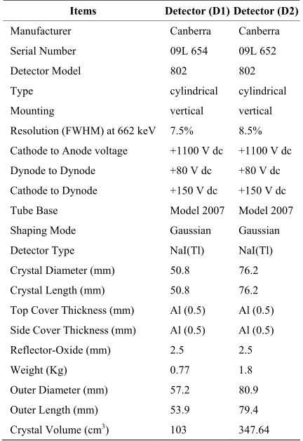
which also specified at the 661 keV were used. The de-tails of these detectors setup parameters with acquisition electronics specifications are listed in Table 1 supported by the (serial & model) number.
In these measurements, the standard point sources
241Am, 133Ba, 152Eu, 137Cs and 60Co where used (these
point sources were purchased from The Physikalisch- Technische Bundesanstalt (PTB) in Braunschweig and Berlin). The certificates give the sources activities and their uncertainties for (PTB) sources are listed in Table 2. The data sheet states values of half lives, photon energies and photon emission probabilities per decay for the all radionuclides used in the calibration process are listed in Table 3, which available from the National Nuclear Data Center Web Page or on the IAEA website.
[image:2.595.56.289.558.639.2]Table 1. Detectors setup parameters with acquisition elec-tronics specifications for Detector (D1) and Detector (D2).
Items Detector (D1) Detector (D2)
Manufacturer Canberra Canberra
Serial Number 09L 654 09L 652 Detector Model 802 802
Type cylindrical cylindrical
Mounting vertical vertical
Resolution (FWHM) at 662 keV 7.5% 8.5% Cathode to Anode voltage +1100 V dc +1100 V dc Dynode to Dynode +80 V dc +80 V dc
Cathode to Dynode +150 V dc +150 V dc Tube Base Model 2007 Model 2007 Shaping Mode Gaussian Gaussian
Detector Type NaI(Tl) NaI(Tl) Crystal Diameter (mm) 50.8 76.2 Crystal Length (mm) 50.8 76.2 Top Cover Thickness (mm) Al (0.5) Al (0.5)
Side Cover Thickness (mm) Al (0.5) Al (0.5) Reflector-Oxide (mm) 2.5 2.5 Weight (Kg) 0.77 1.8
Outer Diameter (mm) 57.2 80.9 Outer Length (mm) 53.9 79.4
[image:3.595.307.538.122.304.2]Crystal Volume (cm3) 103 347.64
Table 2. PTB point sources activities and their uncertain-ties.
PTB-Nuclide Activity (KBq) Reference Date Uncertainty (KBq)
241Am 259.0 ±2.6
133Ba 275.3 ±2.8
152Eu 290.0 ±4.0
137Cs 385.0 ±4.0
60Co 212.1
00:00 Hr 1. June 2009
±1.5
soft enough to be absorbed completely before entering the detector [10]. The source-detector separations start from 20 cm to neglect the coincidence summing correc-tion.
The spectrum was recorded as example P4D1, where, P, refers to the source type (point) measured on detector (D1) at the distance number (4), which means (h = 20 cm).
The spectrum acquired with winTMCA32 software made by ICx Technologies, were analyzed with (Genie 2000 data acquisition and analysis software) made by Canberra using its automatic peak search and peak area calculations, along with changes in the peak fit using the interactive peak fit interface when necessary to reduce
Table 3. Half lives, photon energies and photon emission probabilities per decay for the all radionuclide’s used in this work.
PTB-Nuclide Energy (keV) Probability % Emission Half Life (Days)
241Am 59.52 35.9 157861.05
133Ba 80.99 34.1 3847.91
121.78 28.4 244.69 7.49 344.28 26.6 778.9 12.96 964.13 14.0 152Eu 1408.01 20.87 4943.29
137Cs 661.66 85.21 11004.98
1173.23 99.9 60Co
1332.5 99.982 1925.31
the residuals and error in the peak area values. The live time, the run time and the start time for each spectrum were entered in the spread sheets. Those sheets were used to perform the calculations necessary to generate the experimental full energy peak efficiency (FEPE) curves with their associated uncertainties as a function of the photon energy for all cylindrical NaI(Tl) detectors listed in Table 1 and with different point sources posi-tions.
The ETNA program used to convert the Full Energy Peak Efficiency (FEPE) curve from point sources at po-sition (P4) to the FEPE at popo-sitions (P5, P6, P7, P8, P9 and P10). These calculations extended for two cylindrical NaI(Tl) detectors (D1 & D2).
4. Results and Discussion
This part shows the comparisons between the efficiency transfer theoretical method (ETTM) with the experimen-tal work which is done at Younis S. Selim Laboratory for Radiation Physics, Faculty of Science, Alexandria Uni-versity. This laboratory uses several coaxial NaI(Tl) scintillation detectors (5.08 × 5.08 cm2 and 7.62 × 7.62
cm2) which used in the present work. The detectors were
calibrated by measuring low activity point sources, which previously described. The theoretical Full Energy Peak Efficiency (FEPE) can obtain as described in Equation (3).
[image:3.595.55.288.468.551.2]ciency calculations was the uncertainties of the activities of the standard source solutions. Coincidence summing effects were negligible in the reference measurement geometries.
Cal meas meas
% 100
(10)
where, εCal and εmeas, are the calculated and
experimen-tally measured efficiencies, respectively. The uncertainty in the full-energy peak efficiency, σε, was given by:
The measured efficiency values as a function of the photon energy, ε(E), for all NaI(Tl) scintillation detectors
were calculated by: 2 2 2
2 2
A P
A P N
N2
(13)
i SN E
E C
T A P E
(11) where, σA, σP, and, σN, are the uncertainties associated
with the quantities, AS, P(E), and, N(E), respectively,
as-suming that the only correction made is due to the source activity decay.
where, N(E), is the number of counts in the full-energy peak which can be obtained using Genie 2000 software, T, is the measuring time (in second), P(E), is the photon emission probability at energy, E, AS, is the radionuclide
activity and, Ci, are the correction factors due to dead
time, radionuclide decay.
In order to study the effect of the detector volume, and the source-to-detector distance on the full-energy peak efficiency of NaI(Tl) detectors (D1 and D2), comparing the measured efficiency for different source detector ar-rangement were done.
In these measurements of low activity sources, the dead time always less than 3%, so the corresponding factor was obtained simply using ADC live time. The statistical uncertainties of the net peak areas were smaller than 1.0% since the acquisition time was long enough to get number of counts at least 10,000 counts. The back-ground subtraction was done. The decay correction, Cd,
for the calibration source from the reference time to the run time was given by:
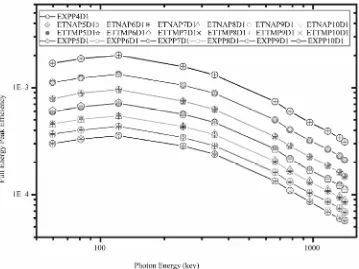
For D1 the maximum measured FEPE value of detec-tor measured with point sources placed at P4 and the minimum one which measured at P10. Also we found that D2 obey the same behavior, by comparison between D1 and D2 results we found that D2 FEPE is greater than it for D1, P4D2 has the maximum FEPE and P10D1 has the minimum one as shown in Figure 2. This phenome-non related to that, the gamma-ray intensity emanating from a source falls off with the distance according to the inverse square law. In addition to the larger detector in dimensions is the more efficient one.
T d
C e (12)
where, λ, is the decay constant and, ΔT, is the time inter-val over which the source decays corresponding to the
run time. The main source of uncertainty in the effi- The full-energy peak efficiency calculated by the pre-
(b)
Figure 2. Comparison between various experimental (FEPE) efficiency results for measured point sources at different posi-tions (P4 up to P10) by using detectors (D1 and D2). (a) Detector (D1) Experimental results; (b) Detector (D2) Experimental results.
Figure 3. Comparison between ETNA, ETTM, and experimental (FEPE) efficiencies for conversion from point sources at (P4 up to P10) using (D1) detector.
sent ETTM and ETNA program over a wide energy range and have been tested against various data sets ob-tained by the experimental method using point sources
[image:5.595.120.479.389.658.2]The efficiency of the detectors is higher at low source energies (absorption coefficient is very high) and de-creases as the energy inde-creases (fall off in the absorption coefficient) because the photoelectric is dominant below 100 keV, which mean in other words that it is higher for the bigger detector than the smaller one and it is higher for lower source energy than higher source energy be-cause of the dominance of the photoelectric at lower source energies.
The present work provides a great understanding to several aspects of gamma-ray spectroscopy and will pro-vide us with useful tools ETTM for efficiency calculation for detectors (D1 and D2). This method constitute good approach for the efficiency computation for laboratory routine measurements and can save time in avoiding ex-
perimental calibration for different position geometries, where the values of the efficiency calculations using ETTM was compared with the measured ones Tables 4 and 5.
5. Conclusion
[image:6.595.58.538.301.734.2]This work show the way to a simple method (ETTM) to compute the full-energy peak efficiency over a wide en-ergy range, which deal with different detector types using isotropic axial point sources. The present work can be extensive to calculate the FEPE for more complicated geometries. The discrepancies in wide-ranging for all the measurements were found to be less (8%) in case of ETNA program and our ETTM expressions with the
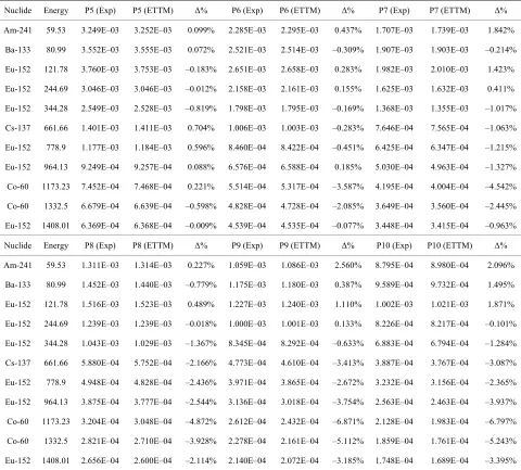
Table 4. Point sources theoretical full energy peak efficiency for D1 (ETTM), and the Discrepancy percentage (Δ%) with ex-perimental values.
Nuclide Energy P5 (Exp) P5 (ETTM) Δ% P6 (Exp) P6 (ETTM) Δ% P7 (Exp) P7 (ETTM) Δ%
Am-241 59.53 3.249E–03 3.252E–03 0.099% 2.285E–03 2.295E–03 0.437% 1.707E–03 1.739E–03 1.842%
Ba-133 80.99 3.552E–03 3.555E–03 0.072% 2.521E–03 2.514E–03 –0.309% 1.907E–03 1.903E–03 –0.214%
Eu-152 121.78 3.760E–03 3.753E–03 –0.183% 2.651E–03 2.658E–03 0.283% 1.982E–03 2.010E–03 1.423%
Eu-152 244.69 3.046E–03 3.046E–03 –0.012% 2.158E–03 2.161E–03 0.155% 1.625E–03 1.632E–03 0.411%
Eu-152 344.28 2.549E–03 2.528E–03 –0.819% 1.798E–03 1.795E–03 –0.169% 1.368E–03 1.355E–03 –1.017%
Cs-137 661.66 1.401E–03 1.411E–03 0.704% 1.006E–03 1.003E–03 –0.283% 7.646E–04 7.565E–04 –1.063%
Eu-152 778.9 1.177E–03 1.184E–03 0.596% 8.460E–04 8.422E–04 –0.451% 6.425E–04 6.347E–04 –1.215%
Eu-152 964.13 9.249E–04 9.257E–04 0.088% 6.576E–04 6.588E–04 0.185% 5.030E–04 4.963E–04 –1.327%
Co-60 1173.23 7.452E–04 7.468E–04 0.221% 5.514E–04 5.317E–04 –3.587% 4.195E–04 4.004E–04 –4.542%
Co-60 1332.5 6.679E–04 6.639E–04 –0.598% 4.828E–04 4.728E–04 –2.085% 3.649E–04 3.560E–04 –2.445%
Eu-152 1408.01 6.369E–04 6.368E–04 –0.009% 4.539E–04 4.535E–04 –0.077% 3.448E–04 3.415E–04 –0.963%
Nuclide Energy P8 (Exp) P8 (ETTM) Δ% P9 (Exp) P9 (ETTM) Δ% P10 (Exp) P10 (ETTM) Δ%
Am-241 59.53 1.311E–03 1.314E–03 0.227% 1.059E–03 1.086E–03 2.560% 8.795E–04 8.980E–04 2.096%
Ba-133 80.99 1.452E–03 1.440E–03 –0.779% 1.175E–03 1.180E–03 0.387% 9.589E–04 9.732E–04 1.495%
Eu-152 121.78 1.516E–03 1.523E–03 0.489% 1.227E–03 1.240E–03 1.110% 1.002E–03 1.021E–03 1.871%
Eu-152 244.69 1.239E–03 1.239E–03 –0.018% 1.000E–03 1.001E–03 0.133% 8.226E–04 8.217E–04 –0.101%
Eu-152 344.28 1.043E–03 1.029E–03 –1.367% 8.345E–04 8.292E–04 –0.633% 6.883E–04 6.794E–04 –1.284%
Cs-137 661.66 5.880E–04 5.752E–04 –2.166% 4.773E–04 4.610E–04 –3.413% 3.887E–04 3.767E–04 –3.087%
Eu-152 778.9 4.948E–04 4.828E–04 –2.436% 3.971E–04 3.865E–04 –2.672% 3.232E–04 3.156E–04 –2.365%
Eu-152 964.13 3.875E–04 3.777E–04 –2.544% 3.136E–04 3.018E–04 –3.754% 2.563E–04 2.463E–04 –3.937%
Co-60 1173.23 3.204E–04 3.048E–04 –4.872% 2.612E–04 2.432E–04 –6.871% 2.128E–04 1.983E–04 –6.797%
Co-60 1332.5 2.821E–04 2.710E–04 –3.928% 2.278E–04 2.161E–04 –5.112% 1.859E–04 1.761E–04 –5.243%
Figure 4. Comparison between ETNA, ETTM, and experimental (FEPE) efficiencies for conversion from point sources at (P4 up to P10) using (D2) detector.
Table 5. Point sources theoretical full energy peak efficiency for D2 (ETTM), and the Discrepancy percentage (Δ%) with ex-perimental values.
Nuclide Energy P5 (Exp) P5 (ETTM) Δ% P6 (Exp) P6 (ETTM) Δ% P7 (Exp) P7 (ETTM) Δ% Am-241 59.53 1.122E–03 1.133E–03 0.951% 7.868E–04 7.849E–04 –0.238% 5.963E–04 6.094E–04 2.188%
Ba-133 80.99 1.234E–03 1.250E–03 1.313% 8.911E–04 8.727E–04 –2.068% 6.625E–04 6.715E–04 1.358% Eu-152 121.78 1.335E–03 1.349E–03 1.058% 9.611E–04 9.453E–04 –1.647% 7.146E–04 7.236E–04 1.270% Eu-152 244.69 1.054E–03 1.054E–03 0.024% 7.481E–04 7.421E–04 –0.809% 5.644E–04 5.654E–04 0.183% Eu-152 344.28 8.864E–04 8.825E–04 –0.435% 6.263E–04 6.222E–04 –0.659% 4.738E–04 4.731E–04 –0.144% Cs-137 661.66 4.999E–04 4.959E–04 –0.800% 3.476E–04 3.507E–04 0.875% 2.668E–04 2.658E–04 –0.398% Eu-152 778.9 4.038E–04 4.024E–04 –0.351% 2.847E–04 2.848E–04 0.010% 2.153E–04 2.156E–04 0.165% Eu-152 964.13 3.195E–04 3.166E–04 –0.908% 2.249E–04 2.242E–04 –0.290% 1.695E–04 1.696E–04 0.061% Co-60 1173.23 2.647E–04 2.620E–04 –1.012% 1.863E–04 1.857E–04 –0.318% 1.396E–04 1.404E–04 0.517% Co-60 1332.5 2.295E–04 2.268E–04 –1.162% 1.616E–04 1.609E–04 –0.432% 1.217E–04 1.215E–04 –0.116% Eu-152 1408.01 2.093E–04 2.080E–04 –0.590% 1.473E–04 1.475E–04 0.181% 1.117E–04 1.114E–04 –0.212% Nuclide Energy P8 (Exp) P8 (ETTM) Δ% P9 (Exp) P9 (ETTM) Δ% P10 (Exp) P10 (ETTM) Δ% Am-241 59.53 4.590E–04 4.638E–04 1.047% 3.683E–04 3.733E–04 1.369% 3.004E–04 2.970E–04 –1.122%
Ba-133 80.99 5.067E–04 5.108E–04 0.812% 4.004E–04 4.090E–04 2.152% 3.298E–04 3.307E–04 0.275% Eu-152 121.78 5.458E–04 5.503E–04 0.821% 4.348E–04 4.390E–04 0.967% 3.557E–04 3.586E–04 0.810% Eu-152 244.69 4.325E–04 4.297E–04 –0.652% 3.422E–04 3.413E–04 –0.264% 2.847E–04 2.818E–04 –0.997% Eu-152 344.28 3.634E–04 3.594E–04 –1.108% 2.856E–04 2.850E–04 –0.233% 2.388E–04 2.364E–04 –1.004% Cs-137 661.66 2.042E–04 2.018E–04 –1.205% 1.619E–04 1.594E–04 –1.548% 1.340E–04 1.334E–04 –0.464% Eu-152 778.9 1.661E–04 1.637E–04 –1.485% 1.305E–04 1.292E–04 –0.951% 1.090E–04 1.083E–04 –0.661% Eu-152 964.13 1.313E–04 1.287E–04 –1.950% 1.035E–04 1.015E–04 –1.909% 8.603E–05 8.531E–05 –0.839% Co-60 1173.23 1.084E–04 1.065E–04 –1.738% 8.598E–05 8.395E–05 –2.363% 6.864E–05 7.067E–05 2.952% Co-60 1332.5 9.408E–05 9.220E–05 –1.996% 7.456E–05 7.263E–05 –2.593% 5.963E–05 6.122E–05 2.662% Eu-152 1408.01 8.582E–05 8.455E–05 –1.471% 6.842E–05 6.659E–05 –2.678% 5.705E–05 5.616E–05 –1.562%
[image:7.595.57.538.442.732.2]experimental values at all energy region.
6. Acknowledgements
The authors would like to introduce a special thanks to Prof. Mahmoud I. Abbas,Faculty of Science, Alexandria University, for fruitful help.
REFERENCES
[1] Y. S. Selim and M. I. Abbas, “Source-Detector Geomet-rical Efficiency,” Radiation Physics and Chemistry, Vol. 44, No. 1-2, 1994, pp. 1-4.
doi:10.1016/0969-806X(94)90093-0
[2] Y. S. Selim and M. I. Abbas, “Direct Calculation of the Total Efficiency Cylindrical Scintillation Detectors for Extended Circular Sources,” Radiation Physics and Che- mistry, Vol. 48, No. 1, 1996, pp. 23-27.
doi:10.1016/0969-806X(95)00047-2
[3] V. Tim, B. Vodenik and M. Necemer, “Efficiency Trans-fer between Extended Sources,” Applied Radiation and Isotopes, Vol. 68, No. 12, 2010, pp. 2352-2354.
doi:10.1016/j.apradiso.2010.05.010
[4] M. C. Lepy, et al., “Intercomparison of Efficiency Trans-fer Software for Gamma-Ray Spectrometry,” Applied Ra-diation and Isotopes, Vol. 55, No. 4, 2001, pp. 493-503. [5] T. Vidmar, et al., “An Intercomparison of Monte Carlo
Codes Used in Gamma-Ray Spectrometry,” Applied Ra-diation and Isotopes, Vol. 66, No. 6-7, 2008, pp. 764-768. doi:10.1016/j.apradiso.2008.02.015
[6] F. Piton, et al., “Efficiency Transfer and Coincidence Summing Corrections for Gamma-Ray Spectrometry,”
Applied Radiation and Isotopes, Vol. 52, No. 3, 2000, pp. 791-795. doi:10.1016/S0969-8043(99)00246-8
[7] S. Jovanovic, et al., “ANGLE: A PC-Code for Semicon-ductor Detector Efficiency Calculations,” Radiation Phy- sics and Chemistry, Vol. 218, No. 1, 1997, pp. 13-20. [8] M. S. Badawi, “Faculty of Science,” Ph.D. Thesis,
Alex-andria University, AlexAlex-andria, 2009.
[9] M. I. Abbas, “HPGe Detector Absolute Full-Energy Peak Efficiency Calibration including Coincidence Correction for Circular Disc Sources,” Journal of Physics D: Applied Physics, Vol. 39, No. 18, 2006, pp. 3952-3958.
doi:10.1088/0022-3727/39/18/005
[10] K. Debertin and U. Schotzig, “Coincidence Summing Cor- rections in Ge(Li)-Spectrometry at Low Source-to-De-tector Distances,” Nuclear Instruments and Methods, Vol. 158, 1979, pp. 471-477.