A Comparison of Coherence Based Acoustic Source Identification Techniques

Twelfth International Congress on Sound and Vibration

A Comparison of Coherence Based Acoustic Source

Identification Techniques

Gareth J. Bennett and John A. Fitzpatrick

Department of Mechanical and Manufacturing Engineering Trinity College Dublin

Dublin 2, Ireland

[email protected]

Abstract

Four techniques of source identification are examined and the performance of each evaluated with experimental data. The procedures are all frequency domain methods and depend to some extent on the coherence function. The Coherent Output Spectrum (COS) technique, reported by Bendat and Halvorsen [1], requires a measure of at least one input and one output irrespective of the number of inputs. The Signal Enhance-ment(SE) technique, developed by Chung [2], requires three output measurements for the identification of a single unmeasured source. The Conditional Spectral Analysis (CSA) technique, proposed by Hsu and Ahuja [3], is a combination of these, where one of two inputs is monitored with three output measurements. The final technique considered is applicable to a system which contains any number of inputs. For this, no input measure is required and the number of output measurements is a function of the number of inputs, as reported by Minami and Ahuja [4]. A series of tests have been conducted to examine the efficacy of each of the procedures for specific applications.

INTRODUCTION

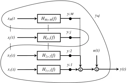
Figure 1. Multiple Source Acoustic Measurement For the case where it is not possible to

turn individual sources off without ef-fecting the behaviour of the others, the challenge is to decompose the measure-ment signal into its constituent parts. For acoustic sources that are consid-ered to be stationary random processes with zero mean and where systems are constant-parameter linear systems, figure 1, a mutiple-input/single-output model, can be used to represent the system. The extraneous noise term,n(t), accomodates all deviations from the model, such as

acoustic sources greater thanM which are unaccounted for, linear operations, non-stationary effects, acquisition, instrument and mathematical noise along with unsteady pressure fluctuations local to the sensor, such as flow or hydrodynamic noise.

IDENTIFICATION TECHNIQUES

In real situations extraneous noise may be measured at the input and/or output of the system. Figure 2 shows the general model where u(t) passes through the system to produce the true outputv(t). m(t) and n(t) represent the extraneous noise measured withinx(t)andy(t). The coherence function, which is the principle tool used in these techniques, is defined as:1

γ_xy2 = |Gxy|

2

GxxGyy

≤ 1 (1)

If the coherence function is greater than zero but less than unity, one or more of the three possible physical situations exist: 1) extraneous Noise is present in the measurements; 2) the system relatingx(t) and y(t)is not linear; 3)y(t)is an output due to an input

x(t)as well as to other inputs.

Coherent Output Spectrum

A particular case of interest is where there is no input noise and the output noise is uncorrelated with both the input and output measurements, viz. x(t) = u(t), y(t) =

v(t) +n(t)andGxn =Gvn = 0. Given these conditions, the following expressions can be expressed:

Gvv =

|Gxv|

2

Gxx

= |Gxy|

2

Gxx

=Gyyγ

2

xy (2)

1_{The frequency dependent notation will be omitted for simplicity of representation.}

Gnn =Gyy−

|Gxy|

2

Gxx

=Gyy(1−γ

2

xy) (3)

The productGyyγ

2

xy, as discussed by Bendat [1], is called the coherent output spectrum andGyy(1−γ

2

xy)is termed the noise output spectrum. This is a highly significant result as we see that the unmeasurable component ofywhich is attributable to the inputxcan be determined from the measured records. We can see, as presented graphically in figure 1, that the coherent output spectrum decomposes the output into one part correlated with the input, and a second uncorrelated with the input, viz.,y(t) = y:j(t) +y·j(t).

The principle limitation of the COS technique is that a measure of one source of interest alone, i.e. a source which is uncorrelated with other inputs to the output measurement, may be difficult to obtain and that it in turn may also contain extraneous noise. When this is the case, the calculated coherent output spectrum Gv0v0 may be significantly less than the actualGvv as illustrated in equation (4).

Gv0v0 =γ

2

x0yGyy =Gvv

Gxx

G_xx +G_mm ≤Gvv (4) The techniques in [5] and [6] each use the COS technique to measure the core noise contribution of a gas turbine or aircraft engine to a farfield measurement. This ability to measure the core noise continues to receive attention because, although the core noise is typically a less significant engine acoustic source, it sets an acoustic threshold below which the engine noise may not pass despite the large reduction in jet and fan noise in recent years. In addition, the current trend towards high-bypass en-gines and low Nox combusters will result in the core noise becoming a more significant source which will need to be measured and suppressed.

Signal Enhancement

As shown in equation (4), an input measurement which contains noise will result in an erroneously low coherent output spectrum. If the coherence between the input and output is high, one may be confident in the calculated COS. However, if the coherence is low, then it is difficult to establish whether this is due to noise in the output measure-ment only or whether there is noise present in the input also. Chung [2] developed a technique which can accomodate for the situation as seen in the model in figure 2 if at least three output measurements are available. If three measurements each contain the same correlated source, a new model may be depicted, as in figure 3.

With regard to figure 3, Chung [2] and Bendat and Piersol [7] demonstrate that the contribution of the input to each of the outputs can be calculated using only the three output measurements. ForGy2, for example, the following can be derived:

Gy2:x=

|γy1y2||γy2y3|

|γy1y3|

Gy2y2 =

|Gy1y2||Gy2y3|

|Gy1y3|

Figure 2. Input/Output Relationship with Noise Figure 3. Signal Enhancement Model

Conditional Spectral Analysis

One of the limitations of the SE technique is that for measurement locations within the same pressure field, the technique may be applied when there is a single correlated source between the records. Minami and Ahuja [4] discuss the errors resulting from using the Signal Enhancement technique when two sources, as opposed to only one source, are buried within extraneous noise. For the situation where there are only two correlated sources, and a measure of one of them is attainable, the COS and the SE techniques may be used in conjunction with each other and with conditional spectral analysis to successfully identify both sources and the extraneous noise. This approach is presented by Hsu and Ahuja [3].

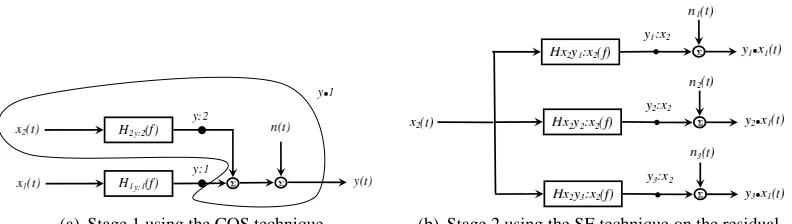
The problem case is illustrated in figure 4(a). The first stage consists of separating out the part correlated with the measurable source, using the COS technique, and thus identifies its contribution. The second stage uses a partial coherence form of the SE technique on the residual to remove the extraneous noise, see figure 4(b). A measure of at least one of only two sources and three output measurements are required for this technique.

(a) Stage 1 using the COS technique (b) Stage 2 using the SE technique on the residual

Figure 4. Conditional Spectral Analysis Technique

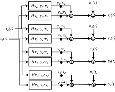
System of Non-Linear Equations

The techniques discussed above set out how up to two distinct sources can be iden-tified from within a measurement containing them and uncorrelated noise. However, a measure of at least one of the sources, which itself may or may not contain further

uncorrelated noise, is necessary when more than one source is present. Minami and Ahuja [4] report a technique where an unlimited number of uncorrelated noise sources can be identified from within extraneous noise when no source is measureable: only output measurements are required the number of which is a function of the number of sources. The method consists of defining relationships between the various contri-butions at each microphone and then solving numerically the subsequent system of non-linear equations for the unknowns of interest. Matlab’s fsolve function, from its

Optimisation Toolbox, was used to solve the system of non-linear equations. The

func-tion was evoked as a funcfunc-tion of frequency.

The Two Test Procedure

The limitation of the SE technique is that only one correlated source between the mea-surements may be present. For the Non-Linear technique, in principle, any number of sources can be present. However, an initial decision has to be made as to the num-ber in order to formulate the necessary system of equations needed for the identifica-tion. A simple procedure is presented here which can be used to verify the number of sources assumed. The procedure, which will be called “The Two Test Procedure”, entails performing an identification with three microphones, M1, M2 and M3 and then performing a second identification where two of the microphones are re-used in conjunction with a fourth microphone located elsewhere, i.e.M1,M2andM4. For fre-quency ranges where the identifications lead to similar results for one of the common microphones, it can be deduced that there is only one significant source. If the results differ however, then there must be other significant sources present in that range.

EXPERIMENTAL SETUP

In order to investigate the performance of these four existing techniques and this new procedure, experiments were carried out using real acoustic data acquired from micro-phones in an acoustic field where the noise sources were small speakers.

Figure 5. Schematic of the Test Set-up The objective of the techniques was to

identify the spectra of the individual sources measured at each microphone lo-cation in the presence of extraneous noise and/or other source fields. In order to have a “solution” against which the per-formance could be evaluated, a measure-ment at the microphones of each source in turn, with the other sources turned off, was recorded.

A schematic of the geometric lay-out of the experiment is shown in figure

and speakers were all located close together, with the microphones mounted directly on the ground, hence reducing reflections from it, in order to ensure coherences close to unity between the microphones for the individual sources.

The extraneous noise terms were incorporated by adding different random noise to each of the measured signals after acquisition. The addition of the noise at the soft-ware stage helped ensure that it was uncorrelated between the signals. The coherences between the various noise signals generated were verified to be close to zero.

In order to evaluate the performance of the techniques over a wide frequency range the speakers were excited with broadband noise. Three separate noise generators, band passed [250Hz-8kHz], ensured three completely uncorrelated source signals. In each of the tests, an acquisition of the voltage feeding the speakers was taken. These readings,x1,x2 andx3 represent a pure measurement of the acoustic source.

Data acquisistion parameters: For each of the channels, a sample rate of 12.5kHz was used to acquire 20 seconds worth of data. For averaging, a block length of 1024 points (bandwidth of 12.2Hz) was used with a 50% overlap and a hanning window.

EXPERIMENTAL RESULTS

Figure 6 shows a sample single source model for speaker x1 only, whereas figure 7

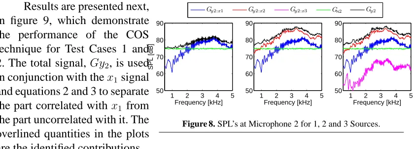
depicts a model where two speakers both contribute to the pressure field. These set-ups will be referred to as Test Case 1 and Test Case 2. Some sample auto-spectra (PSD’s) are given for microphone 2 in figure 8. In each of the three plots an additional speaker is turned on. After each acquisition, random noise (shown in green) was added to the signal measured by the microphone. Thus, the black plot is the “total” signaly2used in

the techniques. The pre-recorded individual speaker measurements are superimposed onto the plots to illustrate their contribution to the total signal. It is these spectra that the techniques, operating on only the measured spectra plus noise, attempt to identify.

Figure 6. Test Case 1 Figure 7. Test Case 2

1 2 3 4 5 50

60 70 80 90

Frequency [kHz]

SPL [dB]

1 2 3 4 5

50 60 70 80 90

Frequency [kHz]

1 2 3 4 5

50 60 70 80 90

Frequency [kHz]

Gy2:x1 Gy2:x2 Gy2:x3 G_n2 Gy2

Figure 8. SPL’s at Microphone 2 for 1, 2 and 3 Sources. Results are presented next,

in figure 9, which demonstrate the performance of the COS technique for Test Cases 1 and 2. The total signal,Gy2, is used

in conjunction with thex1signal

and equations 2 and 3 to separate the part correlated withx1 from

the part uncorrelated with it. The overlined quantities in the plots are the identified contributions.

Figure 11(a) presents results fory2for both the SE and Non-Linear techniques for

Test Case 1 using microphonesM1,M2andM3initially and thenM1, M2andM4

in order to illustrate the “Two Test Procedure”. Figure 11(b) shows the same analysis sfor Test Case 2.

Hsu and Ahuja [3] present a very useful variation of the CSA technique where a formulation allows for noise in the source measurement. The block diagram for this model is given in figure 12(a). The assumption here is that the source measurements may contain noise but that it must be uncorrelated with all other measurement noise and inputs. Two such measurements are required. Results for the CSA technique and its variation are presented in figure 10.

DISCUSSION AND CONCLUSIONS

The ability of the COS technique to successfully identify a source buried within extran-ious noise and/or other sources has been demonstrated in figure 9. A direct measure of the source is required. As discussed above, when a pure measurement of the object source is not possible the COS technique will give inaccurate results. Instead the SE or Non-linear techniques can be used for a single source situation. Both techniques perform well, accurately identifying the source and noise contributions to the measure-ment when no measure of the source is available, see figure 11(a). The limitation of the SE technique is that there can only be one correlated source between the microphone measurements. The same limitation applies to the Non-Linear technique formulated for a single source model.

In order to verify the number of sources assumed, the “Two test Procedure” can be used. In figure 11(b) the SE and Non-linear techniques are applied to Test Case 2. Here it can be seen that the results up to approximately 1.5kHz using either M3 or

two sources, albeit one is10dBlarger than the other, that is also identified in this range as opposed to merely the larger of the two. Above this frequency limit, the results are inconclusive.

The benefit of the CSA technique over the COS technique for Test Case 2, for ex-ample, is that it can identify the second source in addition to the noise term, as opposed to just the sum of the two. The first plot in figure 10 shows each contribution to the

y2 measurement individually identified. In the second plot, the same contributions are

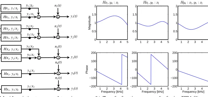
identified, yet in this case a variation of the technique was employed which allowed for extraneous noise in the source measurement. In order to try and replicate this situation, two different windowed linear-phase finite impulse response filters were designed in

M atlaband applied to the measured source signalx1. The magnitude and phase of the

transfer functions betweenx1 and the filtered signals are given in figure 12(b). Also,

shown is the transfer function between the two filtered signals. This is a good physical approximation to the reality as a phase lag between the signals due to their differing lo-cations and magnitude variations would be expected. To these signals, different random noise was added resulting iny4andy5, as per figure 12(a).

Although the results are not presented here, the “Two Test Procedure” was per-formed on CSA technique also. The results show that when a third source, x3, was

turned on, the procedure could be used successfully to verify the number of sources present.

1 2 3 4 5

60 65 70 75 80 85 90

Frequency [kHz]

SPL [dB]

1 2 3 4 5

60 65 70 75 80 85 90

Frequency [kHz]

Gy2:x1 Gy2·x1 Gy2 Gy2:x Gy2·x1

Figure 9. Results for the COS technique for Test Cases 1 and 2.

1 2 3 4 5

60 65 70 75 80 85 90

Frequency [kHz]

SPL [dB]

Gy2:x1 Gy2:x2 Gn2 Gy2 Gy2:x1 Gy2:x2 Gn2

1 2 3 4 5

60 65 70 75 80 85 90

Frequency [kHz]

SPL [dB]

Figure 10. Results for the CSA Technique and its vari-ation for Test Case 2.

ACKNOWLEDGEMENTS

Partly supported by the SILENCE(R) project under EU contract no. G4RD-CT-2001-00500

REFERENCES

1. J. S. Bendat and W. G. Halvorsen, “Noise source identification using coherent output power spectra,” Sound and Vibration, vol. 9, no. 8, pp. 15, 18–24, 1975.

2. J. Y. Chung, “Rejection of flow noise using a coherence function method,” J. Acoust. Soc. Am., vol. 62, no. 2, pp. 388–395, 1977.

1 2 3 4 5 60 65 70 75 80 85

Mics 1,2 & 3

Signal Enhancement

Gy2:x Gn2 Gy2 Gy2:x Gn2

1 2 3 4 5

60 65 70 75 80 85 Non−Linear

1 2 3 4 5

60 65 70 75 80 85

Mics 1,2 & 4

Frequency [kHz]

1 2 3 4 5

60 65 70 75 80 85 Frequency [kHz]

(a) Results for the SE and Non-Linear Techniques for Test Case 1. In the Second Row Mics 1, 2 and 4 are used.

1 2 3 4 5

60 70 80 90

Mics 1,2 & 3

Signal Enhancement

Gy2·n2 Gn2 Gy2 Gy2·n2 Gn2

1 2 3 4 5

60 70 80 90

Non−Linear

1 2 3 4 5

60 70 80 90

Mics 1,2 & 4

Frequency [kHz]

1 2 3 4 5

60 70 80 90

Frequency [kHz]

(b) Results for the SE and Non-Linear Techniques for Test Case 2. In the Second Row Mics 1, 2 and 4 are used.

Figure 11. Comparing the SE and Non-Linear Techniques for Test Cases 1 and 2. The “Two Test Procedure” is used to verify the number of sources.

(a) CSA model with variation to accomodate noise in source signals.

1 2 3 4 5

0 0.5 1 1.5 2 Magnitude

Hx1, y4:x1

1 2 3 4 5

−200 −100 0 100 200 Frequency [kHz] Phase

1 2 3 4 5

0 0.5 1 1.5 2

Hx1, y5:x1

1 2 3 4 5

−200 −100 0 100 200 Frequency [kHz]

1 2 3 4 5

0 0.5 1 1.5 2

Hy4:x1, y5:x1

1 2 3 4 5

−200 −100 0 100 200 Frequency [kHz]

(b) Transfer functions as a result of using FIR1 filters

Figure 12. CSA Technique

3. J. S. Hsu and K. K. Ahuja, “A coherence-based technique to separate ejector internal mixing noise from farfield measurements,” in AIAA/CEAS 4th Aeroacoustics Conference, no. AIAA-98-2296, June 2-4 1998.

4. T. Minami and K. K. Ahuja, “Five-microphone method for separating two different correlated noise sources from farfield measurements contaminated by extraneous noise,” in AIAA/CEAS 9th Aeroacoustics Conference, no. AIAA-03-3261, (South Carolina), May 12-14 2003.

5. A. M. Karchmer, M. Reshotko, and F. J. Montegani, “Measurement of far field combustion noise from a tur-bofan engine using coherence function,” in AIAA 4th Aeroacoustics Conference, no. AIAA-77-1277, (Atlanta, Georgia), October 3-5 1977.

6. A. M. Karchmer, “Conditioned pressure spectra and coherence measurements in the core of a turbofan engine,” Tech. Rep. TM82688, NASA, 1981. AIAA Paper 81-2052.