Dispersion control for multivariate processes - some comparisons

•

.

~

0 ~ . 0

..

.

..

DEPARTMENT OF COMPUTER AND

MATHEMATICAL SCIENCES

Dispersion Control for Multivariate Processes

-Some Comparisons

Pak Fai Tang and Neil Barnett

(66 EQRM 21)

February

,

1996

(AMS

:

62N10)

TECHNICAL REPORT

VICTORIA UNIVERSITY OF TECHNOLOGY

DEPARTMENT OF COMPUTER AND MATHEMATICAL SCIENCES

P 0BOX14428

MCMC

MELBOURNE, VICTORIA 8001

AUSTRALIA

TELEPHONE (03) 9688 4492

FACSIMILE (03) 9688 4050

DISPERSION CONTROL FOR

MULTIVARIATE PROCESSES - SOME

COMPARISONS

PAK FAIT ANG 1 AND NEIL BARNETT 1 Victoria University of Technology

Summary

In Tang and Barnett (1996) some techniques for monitoring and controlling the dispersion of multivariate normal processes based on subgroup data are presented. In

this current paper, comparisons are made between the proposed techniques and

various competing procedures. Simulation results indicate that the proposed

techniques are superior to existing procedures.

Key words : Dispersion control; multivariate normal processes; rational subgroups; statistical performance.

1. Introduction

In Tang and Barnett (1996), some procedures for monitoring and controlling the dispersion of multivariate normal processes based on rational subgroups are

presented for both cases where the in-control value of the process covariance matrix

L

is specified and alternatively unknown in advance of production. Essentially, these

1

Dept of Computer and Mathematical Scie!:lces

techniques involve the aggregation of suitably transformed variables, resulting from

the decomposition of the covariance or some positive definite matrices, in order to

produce control statistics having chi-square distributions under in-control and

normality assumptions. In the present paper, the relative effectiveness of these and

various competing techniques are studied. In addition, the effect of incorporating

independent components from the decomposition, on the control performance, is

examined for the known

L

case. To set the discussion in context, the proposed

control procedures are briefly reviewed in subsequent paragraphs.

Let sj ( L j ) , s*j (L*j) and sv,u (crv,u) be, respectively, the sample

(population) covariance matrix of the first j variables, that of the last j variables and

the vector of sample (population) covariances between the vth and each of the first u

variables. The conditional sample and population variance of the jth variable given the

first j-1 variables are then given by

s~l · 1=S~-S~ - 1S-:-1

1S··1

l• , ...• 1- l 1.1- 1- 1.1- d

2 2 T ~-1

an cr j•l, ... ,j-1

=

cr j - cr j,j-1 LJ j-1 cr j,j-1 ·

-The conditional sample and population covariance matrices of the last p-j+ 1 variables

given the remaining j-l variables are respectively

( )

T (

s

.

.

=

s*

.

-

s

. .

. . . s

.

s-:-

1

s

..

l •... ,p•l, ... ,1-1 p-1+1 1,.:!,-1 P,.:.;!-1 1-l 1,.:!,-1

... s

p,1-l

.

)

-and

L

·

·

=

L*

·

-

cr . . · · · cr .

I,-:

1

cr ..

( )

T (

Page 3

If d and 0 (j = 2, ... , p) denote respectively the vectors of sample and population

- j - j

regression coefficients when each of the last p-j+ 1 variables is regressed on the (j-l)th

variable whilst the remainingj-2 variables are held fixed, these are expressible as

{(s1

·

-1.1

·

s

.

i

)-sT 1

.

2s~12(s

..

2 ... s

.

2)}T

J- ,p 1-;..J- J- t:.!.,-

~-d =--0.---"~

- j S_{J- ,J-}· 1 · 1-S~1_{J- ,]-}· 2S~_J-12S·1 _{J- ,]-}

· 2

,...,

,...,

and

Note that d and 0 should be interpreted as the vectors of unconditional sample

-2 -2

and population regression coefficients when each of the last p-1 variables is regressed

on the 1st variable and these are given by

(s12

slp

r

d

=---

and

-2

respectively. We also use the same notation for distribution functions of Tang and

Barnett (1996).

For a p-variate normal process with presumably known

I.,

the authors

proposed the use of the following control

statistic:-where

2p-l

Tk =

Iz~(k)

j=l

z

.

= <I>-1{x2 ·[(nk -I)SJ.1 .... ,j-1(k) ]} J(k) nk- J 2

() _{1• ,.} . 1 _{. .,)-}. 1

}=2, ... ,p.

Zp+1(k) =<I>-1

{x

2

p-1[(nk-I)Sick)(d -0

)TI.~~

.

p•1(d -0

J]}

... 2(k) - 2 ' " ... 2(k) ... 2

z .

=<I>-1 2 . -1 s~

.

d -0

I,-:-

1 . d -0

{ [ ( ) T (

)~~

'ptj4(k) xp--1+l (fltc ) 1-l•l, ... 1-2(k) ... j(k) ... j ') .... pel, ... 1-1 ... j(k) ... j }=3, ... ,p.

and the subscript k indicates the subgroup number.

In the absence of prior estimates for I, , the suggested control statistic is

defined as

where

and

2p-1

Tk =

IzJck)

j=l

k=2, ...

z.

=

<1>-1[p

.

[

sJ.1 ...

j-l(k) ] ] J(k) nk-J;Nj,k-1 S2

j,k-1 (pooled)

(2)

j=l, ... ,p.

( Sj

1

,k)

s ;,!::.'" - v

~-1

r (

(

n, -1)-l Sj'., ., +

u

~

-

Tl

(

S;'. '"

s ;.!::."

'

-

v

£-1)

(j - l)SJ,k (pooled)

}=2, ... ,p.

The values of S _J, ~ k( _{pooe 1 d) •} U _J, · k and V _j, k can be updated sequentially using the

:-Page 5

2 1 [ 2 2 ]

S j,k(pooled) =

N

N j,k-lS j,k-1 (pooled)

+

(nk - l)S j•l, ... ,j-l(k) j,k

k

where N j,k

=

L

(ni - j) and

sl~O(i)

=

sl~i)'

i=l

and

Note that for both cases,

{Tk}

is a sequence of independent and identically distributed

(i.i.d) chi-square variables with 2p-l degrees of freedom under the in-control and

normality assumption. Thus, unlike other competing procedures, statistically valid

control limits can be easily obtained for the resulting charts. Note also that since any

instability in

I.

is likely to result in unusually large values in the

Tk

's, it is suggested

using only the upper control limit.

2. Comparisons

In this section, the relative performance of the proposed techniques are

tested against some existing procedures. For the case where I, is assumed known,

comparison is made between the proposed technique, the modified likelihood ratio

test (MLRT), the

ISl

112 charting technique as well as a possible method based on

principal components. The first two charting procedures to be used in the comparison

appear to be the most widely discussed techniques for monitoring the dispersion of

included merely because it appears to be a reasonable technique in situations where

principal components possess meaningful physical interpretations. In fact, as stated in

Jackson (1989), this phenomenon is very common in industrial situations. In addition,

Crosier (1988) has identified situations where ' ... if the mean shifts, it does so along

the major axis .... .'. Under these circumstances, it is expected that changes in

L

may

well occur along some of the principal axes, namely the variances of some principal

components may shift. As for the unknown

L

case, the proposed technique is

compared with the modified likelihood ratio test for the equality of covariance

matrices (MLRTECM) as given, for eg., in Anderson (1984, p.405). For clarity of

subsequent discussion, these techniques are briefly reviewed.

MLRT is an unbiased version of the likelihood ratio test of H₀

:L

=Lo

against HA:L =F-

Lo

with the sample size,

n,

replaced by the number of degrees of

freedom, n -1. This test rejects the null hypothesis H₀ and suggests a departure of

the process covariance matrix from the standard or the known value

Lo

when the

test or control statistic,

w*

exceeds

w;,n,a

where

w*

= -p(n-l)-(n-l)lnlSl+(n-l)lnlLol+Cn-l)tr(Lo1 S ). (3)

a and

w;,n,a

denote respectively the false signal rate and the upper lOOa th

percentage point of W * which depends on p and n. The distributional theory involved

with this technique is prohibitively complicated thus limiting its practicality. Although

w*

can be approximated by a chi-square distribution with p(p+ l) degrees of

2

freedom when n is large, and the exact upper 1 % and 5% percentage points of

w*

Page 7

values of n, these may be of little value in the context of control charting. In practice,

the control or monitoring procedures are likely to be based on samples not sufficiently

large to justify the use of the chi-square approximation. Besides, it may be preferable

to have a control technique with false signal rates considerably smaller than 1 % or

5%. Although MLRT is admissible (see for eg., Giri (1977), p.186), it will be seen

later that this technique is inferior to the proposed technique for all of the cases

considered.

The other competing procedure is based on the use of the square root of the

generalized sample covariance matrix,

ISl

112. The resulting chart can be regarded as a

multivariate analogue of the univariate S chart. When p = 2,

ISl

112 is distributed as a

scaled chi-square variable under the stable or in-control multivariate normality

assumption (Anderson (1984), p.264). Thus, control limits may be set at

I

L

1112 2

LCL = o X2(n-2),a.12

2(n- l)

I

L

1 112 2

and UCL= o X2(n-2),1-a.12

2(n- l) (4)

where x~ 0 denotes the 100 8th percentage point of the chi-square distribution with v '

degrees of freedom. For higher dimensions, Alt et al. (1986) suggested the use of the

3-sigma limits as given by the following formulae :

(5)

The use of this charting technique is ill-advised

because:-(i) it is incapable of detecting changes in

L

such that

IL.I

remains constant.

(ii) the formula (5) above yields negative values for the lower control limit for most

practical values of p and n. If LCL is thus set to zero as suggested by Alt et

al.(1990), this means no protection is provided by the resulting

ISl

112 chart against

a decreasing value in

IL.I .

(iii) the associated false alarm rate is considerably larger than the nominal value of

0.0027 especially when n is relatively small. Refer to Table 1 for the false signal

rates for various practical combinations of p and n. These figures are obtained

based on 10,000 simulation runs except when p = 3 or 4 in which case the entries

are found by numerical integration. Note that, in some cases, the false signal rate

is as large as 2%.

<Insert Table 1 about here>

To illustrate the first two points, consider the case of a trivariate process. In this case,

Page9

subject to the constraint

Thus, it is readily seen that, theoretically, it is possible for

ILi

to remain constant or

even decrease in the presence of process troubles. For example, suppose that

cr₁ = cr₂ =cr₃ =1, p₁₂ = 0.1, p₁₃ = 0.7 and p₂₃ = 0.5 are specified as the in-control

values, but in fact cr₃ ·is 3 times as large as that specified and p₂₃ is .0.7553, then

ILi

remains at the value 0.32. If cr₃ doubles instead, then this results in a smaller value of

ILi.

In either case, the departure is unlikely to be 'picked up' by the

ISl

112 charts

presented by Alt et al.(1986).

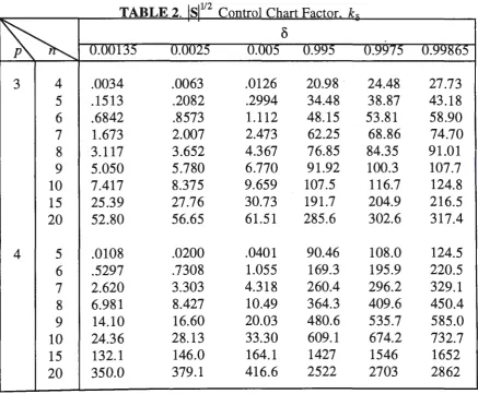
It is perhaps worth noting that, for p = 3 or 4, control limits for the

ISl

112

chart can be obtained numerically at any desired a level. In this case, the control

limits are given by

and UCL= ki-a/2

IL

11/2 2p-2 (n-l)p12 o

where k₅ is a numerical solution to the integral equation,

00

f

G2(n-p) ( kr, / X(p-2)12 )g(p-2)(n-p+2)

(x )dx

= 8.

0

(8)

(9)

The notation gv ( •) and Gv ( •) here denote respectively the probability density and

obtained in this manner using Mathematica version 2.2 (Wolfram (1991)) and is given

to 4 significant digits in Table 2 for p = 3 and 4, and various combinations of

b

and n.

<Insert Table 2 about here>

The last technique considered for the known I, case is aimed at changes of

I, along the principal axes. It involves charting the sum of the standardized variances

for the principal components, abbreviated hereafter as SSVPC, which is known to be

distributed as a scaled chi-square variable under the multi.variate normal assumption

with the hypothesized I, . The value of SSVPC may be calculated from the familiar

equivalent statistic (n-

l)tr(s

I,~1) (see Appendix (A.3)). Note that, unlike all other

control procedures considered in this section, this technique is applicable even in

situations where n::; p. It has also been shown by Kiefer et al.(1965) that it is

admissible. Although separate monitoring of the variances for the different principal

components is possible, this is not considered due to the large number of charts to be

kept when p is large. It is also for meaningful comparison with other techniques

involving a single chart that separate monitoring of the variances is not considered.

However, in practice, it is the recommendation that these individual variances be

retained in order to facilitate the interpretation of out-of-control signals from the

SSVPC charts.

In the absence of prior information about I,, Alt et al.(1990) suggest using

the MLRT and

ISlvz

control charts with the unknown process dispersion parameters

Page 11

data. Under these circumstances, the data used for estimating the unknown

parameters are likely to be either small or moderate data sets. Accordingly, the false

signal rates of the resulting techniques are not fixed but instead vary stochastically

with the parameter estimates. This causes some difficulties when a comparison is to be

made between these and the proposed technique. Thus only MLRTECM, which was

originally proposed in the context of hypotheses testing, is considered.

The criterion for MLRTECM is

(10)

where s(i)' ni and spoooled denote respectively the ith sample covariance matrix, its

associated sample size and the pooled covariance matrix based on the q samples. It

was shown by Anderson (1984) that it is an admissible test if ni > 2p-1, i = l, ... ,q.

For equal sample sizes ni = n , this test rejects the null hypothesis that all the q

samples are drawn from populations with the same covariance matrix if W > Wq,p,n,a.

where Wq,p,n,a. denotes the critical value at the I 00 a% significance level. The upper

5% points of W have been tabulated, for example, in Anderson (1984) for various

combinations of p, q and n. There are two problems with the use of MLRTECM in

the context of SPC. The existing tables for the percentiles of W are incomplete in

regard to other values of p, q, n and a which are required for SPC applications.

Besides, successive values of W are correlated and thus the in-control behaviour of

the resulting technique is somewhat unpredictable. However, it is found that ignoring

this issue does not appear to have any remarkable effect on the overall false signal

rate. Therefore, a reasonable comparison can still be made between this and the

It is shown in Appendix (A. I), (A.3) and (A.4) respectively that the

statistical performance of MLRT, SSVPC and MLRTECM (for a step shift in

L

from

I I

Lo

to

Li)

depend on the eigenvalues,

A

1 , •••

,AP

of L~2

Li

L~2 , or equivalently, of

L~

1

L1

or

L1

L~

1

,

whereas that of the

ISl

112 charting technique depends on

Lo

and

Li

only through the product of these eigenvalues, A₁A_{2 •• •}

AP

(see A.2). Note that

A

₁

A

_{2 \ ..}

AP

represents the ratio of the 'equal-content' volumes of the process

ellipsoids corresponding to

Li

and

Lo

respectively. In addition, Nagao (1967) and

Das Gupta (1969) independently showed that the power function of the MLRT is

monotonically increasing with respect to

!Ai -

~ Vi. Furthermore, note that MLRT,

SSVPC, MLRTECM and

ISl

112 charting procedures are invariant w.r.t. the

transformation

x*

=

rx

+

µ where

r

is any nonsingular matrix. This is not true with

the proposed techniques except when

r

.

is diagonal. By letting

r

=

diag(~

1

.

,

•••

,11; ),

it is readily seen that the values of the proposed statistics are the same whether they

are computed from the covariance or correlation matrix (see A.5 and A.6), and so is

true with the other invariant procedures considered above. However, difficulties arise

when an attempt is made to compare their operating characteristics, since the

statistical properties of the proposed techniques do not appear to be completely

I I

determined by the eigenvalues of

Lo

2

_L

1

Lo

2 • To provide a 'sensible' comparison, it

is therefore necessary to consider several possible combinations of

Lo

and

Li

which

Page 13

of the competing procedures. Note, however, that only

Lo

's m the form of

correlation matrix need to be considered.

A somewhat systematic way of studying the relative performance of the

various competing techniques is to use several arbitrary orthonormal matrices

r

's

that diagonalize

L0

112

Li L0

112 giving the same diagonal matrix of eigenvalues,

A = diag

(A.

_{1 , ••• ,}

A.

P ) • For a given

L

_{0 ,} A and

r ,

L

₁ is then determined from

Li

=L~2rTArL~2.

Amongst others, the orthonormal matrix that diagonalizes

Lo,

r

=

r

₀ is used. This

corresponds to situations where the shift is along the principal axes, namely, the

variances of some principal components either increase or decrease. Under these

circumstances, the eigenvalues of

L0

112

L

₁

L

₀

112 are the ratios ·of variances for the

principal components, after and before the shift, and hence the control performance of

MLRT, MLRTECM, SSVPC and

ISl

112 depend on them (see A.7). Note that if the

eigenvalues of

L

₀

112 L

₁

L

₀

112

are identical, then

L

₁ is the same irrespective of

r.

In

this case,

Li=

A

Lo

where A is the common eigenvalue. This situation may occur in

practice as a consequence of all variances increasing proportionally and the

correlational structure of the variables remaining the same (see Healy (1987)).

The techniques considered for the known

L

case above are compared on the

basis of probability of detecting a persistent shift in the process covariance matrix

from

Lo

to

Li.

It is assumed that this change, as well as the shift in the process

mean vector if any, occur somewhere during the time interval between the sampling of

two adjacent subgroups. Accordingly, the covariance matrices for samples or

mean shift has no effect on this distribution. Of course, if desired, the average run

lengths (ARLs) of the various techniques can be determined as the reciprocals of their

corresponding probabilities of detection. As for the unknown

l:

case, a more

complete profile of the run length (RL) properties is required. This is because the

out-of-control RL distributions of both techniques under consideration are not geometric

so that ARL is not a suitable performance criterion (see Quesenberry (1993)).

Furthermore, since these techniques estimate the in-control dispersion parameters

sequentially from the current data stream and the efficiency of these estimates increase

as more data are incorporated into the computations, it can be expected that their RL

performance depend on when the shift takes place. As such, the relative performance

of MLRTECM and the proposed technique are evaluated based on Pr(RL=S; k) for a

step change in

l:

after the rth subgroup, for various combinations of rand k.

The results for the known

l:

case are tabulated in Tables 3, 4 and 5

respectively for the cases where (p

=

3, n

=

4), (p

=

4, n

=

5) and (p

=

5, n

=

8).

These are based on simulations consisting of 5000 iterations each. Thus, the estimated

maximum standard error of the results is

"

" "

_P_r(_l -_Pr_)

=

0.0071 which occurs when the 5000

estimated probability, Pr= 0.5. For the unknown

l:

case, the results are based on

2000 simulation runs each (with maximum standard error

=

0.0112) and these are

shown in Tables 6, 7 and 8 respectively for (p

=

2, n

=

3), (p

=

3, n

=

4) and (p

=

4, n

= 5). Here, it is assumed that the control procedures are based on subgroups of equal

size, n. The false signal rate associated with each of the control schemes is fixed at

0.0027, in line with the tradional control charting approach. Note that the control

Page 15

of Davis et al.(1971). The control limits for

ISl

112 chart are determined from Table 2

for p

=

3, 4 and by means of simulation consisting of 100,000 iterations for p

=

5 and

n

=

8. Note also that 2-sided control limits with equal significance level on each side are used with SSVPC.

<Insert Tables 3 to 8 about here>

For every set of eigenvalues A.1 , •••

,AP

not enclosed within a bracket, the

probabilities for the proposed techniques are simulated for all possible permutations

and the maximum, median and minimum values are tabulated, except for p = 2 in

which case the median is not applicable. The results for the other control procedures

are unaffected by these permutations. Note that for the cases where the eigenvalues

are identical, the results for the proposed techniques are theoretically the same

irrespective of

Lo

(see next section). As shown in Tables 3, 4 and 5, the proposed

technique is much more powerful than the MLRT and

ISl

112 charting procedures for

all the cases considered. Note that even its worst performance in each case is

significantly better than these procedures. For instance, when p = 3, n = 4 and the

standard deviations of two principal components double, the results for MLRT and

ISl

112

techniques are respectively 0.0564 and 0.1268 whereas the smallest probability

of detection for the proposed procedure is 0.3524. As compared to SSVPC, the

proposed technique is seen to be marginally worst in most cases where some

eigenvalues are greater than 1 whilst others are 1. However, in cases where some

occurs as a result of some but not all of the variances increasing), the proposed

technique is almost always superior. Particularly notable is the situation when p is

large. For instance, whenp = 5, n = 8 and the eigenvalues are (1, 1, 1, 0.1, 10), the

result for SSVPC is 0.7398 whereas those for the proposed technique are 0.7780,

0.8642 and 0.8532 respectively for the different r considered. Note that the exact

probabilities for SSVPC and

ISl

112 charting technique (for p = 3, 4) are obtainable

using standard statistical software and a published program. The program of Davies

(1980) can be used for finding the cumulative probability of SSVPC since the latter is

distributed as a linear combination of independent chi-square variables with

coefficients A._{1 ,. ••}

,A.P

(see A.3). If A._{1 ,. ..}

,A.P

are identical, resulting in a scaled

chi-square distribution, then many statistical software packages currently available can be

used. If p = 3 or 4, the cumulative probability of

ISl

112 can be determined by means of

numerical integration. However, as a partial check of the simulation, the simulation

results for these techniques are included. They are found to agree well with the

theoretical values. For instance, the theoretical probabilities for

ISl

112 and SSVPC are

(0.1333, 0.3828), (0.4575, 0.8873) and (0.7020, 0.9866) for p = 4, n = 5, a= 0.0027

and A._{1 , ..}

.,A.P

all equal to 2.25, 4 and 6.25 respectively. These are very close to the

corresponding figures in Table 4.

As for the comparison for the unknown

L

case, Tables 6, 7 and 8 clearly

reveal that the proposed technique is far superior to MLRTECM irrespective of the

dimension p, the change point r, the eigenvalues A.₁, •••

,A.P

and the direction of the

shift as specified by r . Like the known

L

case, limited comparisons using other

Page 17

It is perhaps worth noting that Calvin (1994) has developed a one-sided test

of covariance matrix with a known null value. However, no attempt has been made to

compare the operating characteristics of this and the proposed technique. A

reasonable comparison cannot be made since the former is specifically designed for

situations where the deviations take the form of

L

=

Lo+

B (B is a symmetric

positive definite matrix) whereas the proposed technique is not meant for any specific

shifts. If the shift is anticipated to be of the form

L

=

Lo+

B, then the

recommendation is to use the former technique.

3. Effect of Aggregation on Control Performance

As presented earlier, the proposed techniques involve the charting of some

aggregate-type statistics formed using independent components resulting from the

partitioning of the covariance matrices. Certainly, if the use of such a statistic incurs

some loss in control performance, then it is preferable to chart the individual

components separately though the improved performance is gained at the expense of

increasing the charting effort. In this section, the effect of such 'aggregation' on the

control performance, is briefly considered for the known

L

case. This effect is

examined by comparing the probabilities of detection by the proposed technique with

that based on the use of the individual components for certain shifts in

L ,

having

equated first their false signal rates. Note that the latter technique, abbreviated

hereafter as the JC technique, involves the plotting of the following statistics

and

(nk - l)SJ.1, ... ,j-1(k) 2

(j_1• . 1 _{, .... 1-}. 1

j = 2, ... ,p. (12)

(13)

(nk-l)S

₁

~_

₁

•

₁

... ₁·_{_2}<k)(d

-0

)TL-

1

·

~

.. p.

1._1(d

-0)

j=3,

.

..

,p. (14)

' ' ,_ j(k) ,_ j ' ' ,_ j(k) ,... j

It may also be of some value to study the control performance of the

technique based on the use of principal components. In the presence of

:L,

it is

reasonable to chart the standardized variances of the principal components (multiplied

by (n-1) each) separately. These are given by the diagonal elements of

I I

(n-l)A₀2

r

0

sr

0A0

2 _{where A}

0 and

rl

denote respectively the diagonal matrix

containing the eigenvalues of

Lo

and the matrix of the corresponding eigenvectors.

For ease of subsequent discussion, this technique is referred to as ISVPC.

Following a shift in the process covariance matrix

L ,

the statistics (11) and

(12) are readily seen to follow some scaled chi-square distribution whereas the

Hotelling

X

2-type statistics in (13) and (14) can be shown to be generally distributed

as linear combinations of independent noncentral chi-square variables (see A.8).

Furthermore, note that the (conditional) independence of these statistics is preserved.

Thus, given the program of Davies (1980), it is possible to determine the overall

probability of 'picking up' any given shift in

L

by the use of these statistics.

However, for mathematical convenience, only a special case is considered, namely,

form:-Page 19

a situation which has been noted earlier. Note that under these circumstances, all the

above statistics are chi-square except for the scalar multiple /.., . The same is true for

the ISVPC technique. Thus, the statistical performance of these and the proposed

technique depends on A (besides p and n) irrespective of

L,

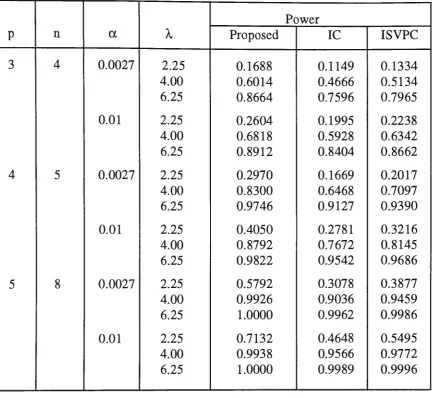
0.

For reasonable comparison, suppose that the significance levels associated

with the control charts for the IC and ISVPC techniques are set to be equal to a* so

that the overall false signal rate, a, for each control scheme is the same as that of the

proposed technique. Accordingly, the a* for both techniques are respectively given

by

*

-'-a

=1-(l-a)2_{p-I and} .

_a

* ~

=l-(l-a)P.

Furthermore, note that both the lower and upper control limits are used with each

* *

chart and these are set at

~

and 1-

~

probability levels respectively. The power of these and the proposed technique are given to 4 decimal places in Table 9 for

various combinations of p, n, /... and

a.

Note that the results for the proposed

technique are obtained by means of 5000 simulation runs. In all these cases, it is

observed that the proposed technique is significantly better than the IC and ISVPC

techniques. It is also seen that ISVPC ranks between the proposed and the IC

technique in performance for all the given shifts. Although no attempt has been made

to study their relative performance thoroughly, the results provide an indication that

incorporating the individual components into a composite statistic in the suggested

<Insert Table 9 about here>

4. Concluding Remarks

Some methods have been presented by Tang and Barnett (1996) for

controlling the dispersion of multivariate normal processes as measured by the

variance-covariance matrix. The one presented for the case with no prior knowledge

of the process parameters is particularly attractive for short production runs and low

volume manufacturing environments. This procedure also enables the monitoring of

new or start-up processes soon after production commences.

A simulation study indicates that the proposed techniques outperform

previously proposed procedures for many sustained shifts in the process covariance

matrix. It has also been demonstrated that the technique presented for the known

.L

case is more powerful in 'picking up' certain shifts than that which involves the

separate charting of the standardized variances of the principal components or the

individual components resulting from the decomposition of the covariance matrices.

In addition, the proposed methods have some practical advantages over the existing

procedures. Besides having a better control over the false alarm rate and the ease of

locating the control limits, the proposed techniques can help identify the nature of

change in the process dispersion parameters. As all multivariate control procedures

are computerised, the complexity of the associated computation should not be an

issue. In fact, almost all standard statistical software packages commercially available

support the implementation of the proposed procedures.

This paper has only considered control procedures based on subgroup data.

Page 21

characteristic at regular time intervals. In this regard, Hawkins (1992), amongst

others, has developed some nonparametric procedures for detecting ramp shifts in

functions of the process dispersion parameters for retrospective and sequential

settings, when the process covariance matrix is either specified or unknown.

However, if the distribution of the observation vectors is known, for example, to be

multivariate normal, a parametric procedure is preferable since better performance is

anticipated. This is an area for future research. Another aspect that warrants

investigation is the robustness of the proposed procedures to departures from the

References

ALT, F. B. and BEDEWI, G. E. (1986). 'SPC of Dispersion for Multivariate Data'.

ASQC Quality Congress Transaction - Anaheim. American Society for Quality

Control, pp. 248-254.

ALT, F. B. and SMITH, N. D. (1990). 'Multivariate Quality Control' in Handbook of

Statistical Methods for Engineers and Scientists, Ed. H.M. Wadsworth,

McGraw-Hill, New York, NY.

ANDERSON, T. W. (1984). An Introduction to Multivariate Statistical Analysis,

2nd ed., John Wiley & Sons, New York, NY.

CALVIN, J. A. (1994). 'One-sided Test of Covariance Matrix with A Known Null

Value'. Communications in Statistics - Theory and Methods 23, pp.3121-3140.

CROSIER, R. B. (1988). 'Multivariate Generalization of Cumulative Sum

Quality-Control Schemes'. Technometrics 30, pp. 291-303.

DAS GUPTA, S. (1969). 'Properties of Power Functions of Some Tests Concerning

Dispersion Matrices of Multivariate Normal Distributions'. Annals of

Mathematical Statistics 40, pp.697-701.

DAVIES, R. B. (1980). "The Distribution of a Linear Combination of

X

2 Random

Variables". Algorithm AS 155, Applied Statistics 29, pp.323-333.

DAVIS, A. W. and FIELD, J. B. F. (1971). 'Tables of Some Multivariate Test

Criteria'. Technical Paper No. 32, C.S.I.R.O, Australia.

GIRI, N. C. (1977). Multivariate Statistical Inference, Academic Press, New York,

NY.

JOHNSON, R. A. and WICHERN, D. W. (1988). Applied Multivariate Statistical

Analysis, 2nd ed., Prentice-Hall, Englewood Cliffs, NJ.

KIEFER, J. and SCHWARTZ, R. (1965). 'Admissible Bayes Character of T2 - and

R2 _{- and Other Fully Invariant Tests for Classical Normal Problems'. Annals}

of Mathematical Statistics 36, pp.747-760.

HAWKINS, D. L. (1992). 'Detecting Shifts in Functions of Multivariate Location and

Covariance Parameters'. Journal of Statistical Planning and Inference 33,

Page 23

HEALY, J. D. (1987). 'A Note on Multivariate CUSUM Procedures'. Technometrics

29, pp.409-412.

JACKSON, J. E. (1991). 'Multivariate Quality Control : 40 Years Later'. in

Statistical Process Control in Manufacturing, Eds. J.B. Keats and D.C.

Montgomery, Marcel Dekker, New York, NY & ASQC Press, Milwaukee,

Wisconsin, pp.123-138.

NAGAO, H. (1967). 'Monotonicity of the Modified Likelihood Ratio Test for a

Covariance Matrix. Journal of Science Hiroshima University Al 31,

pp.147-150.

QUESENBERRY, C. P. (1993). "The Effect of Sample Size on Estimated Limits for

X and X Control Charts". Journal of Quality Technology 25, pp. 237-247.

SRIVASTAVA, M. S. and KHATRI, C. G. (1979). An Introduction to Multivariate

Statistics, Elsevier North Holland, New York, NY.

TANG, P. F. and BARNETT, N. S. (1996). 'Dispersion Control for Multivariate

Processes'. Submitted to Australian Journal of Statistics.

WOLFRAM, S. (1991). Mathematica : A System for Doing Mathematics by

TABLE 1. False Signal Rate of jSj112 Chart with '3-sigma' Limits

~

p

3 4 5 6 7 8 9 10

4 0.0203

5 0.0174 0.0206

6 0.0154 0.0188 0.0203

7 0.0139 0.0172 '

0.0187 0.0219

8 0.0128 0.0159 0.0191 0.0197 0.0202

9 0.0118 0.0149 0.0141 0.0191 0.0199 0.0203

10 0.0111 0.0140 0.0178 0.0192 0.0207 0.0220 0.0205

15 0.0087 0.0110 0.0130 0.0143 0.0157 0.0170 0.0204 0.0180

20 0.0085 0.0093 0.0108 0.0121 0.0148 0.0166 0.0164 0.0140 i

25 0.0071 0.0079 0.0108 0.0123 0.0125 0.0121 0.0124 0.0169

30 0.0056 0.0075 0.0106 0.0111 0.0098 0.0119 0.0137 0.0114

112

TABLE 2. S Control Chart Factor

3 4 .0034 .0063 .0126 20.98 24.48 27.73

5 .1513 .2082 .2994 34.48 38.87 43.18

6 .6842 .8573 1.112 48.15 53.81 58.90

7 1.673 2.007 2.473 62.25 68.86 74.70

8 3.117 3.652 4.367 76.85 84.35 91.01

9 5.050 5.780 6.770 91.92 100.3 107.7

10 7.417 8.375 9.659 107.5 116.7 124.8

15 25.39 27.76 30.73 191.7 204.9 216.5

20 52.80 56.65 61.51 285.6 302.6 317.4

4 5 .0108 .0200 .0401 90.46 108.0 124.5

6 .5297 .7308 1.055 169.3 195.9 220.5

7 2.620 3.303 4.318 260.4 296.2 329.1

8 6.981 8.427 10.49 364.3 409.6 450.4

9 14.10 16.60 20.03 480.6 535.7 585.0

10 24.36 28.13 33.30 609.1 674.2 732.7

15 132.1 146.0 164.1 1427 1546 1652

Page 25

TABLE 3. Power Comparison of Proposed, MLRT,

ISl

112 and SSVPC Charting

Techniques for p = 3, n = 4 and a= 0.0027.

Eigenvalues _Power

of

I.

₀

1

I.

₁ MLRT

1s1112

SSVPC PR1JP(1sl-in a

Max Med Min

2.25, 1, 1 _{0.0030 0.0096 0.0334}

_*

_{0.0366 0.0240 0.0230}

t 0.0350 0.0296 0.0244

:j: 0.0402 0.0264 0.0250 2.25, 2.25, 1 0.0050 0.0348 0.1060 0.0908 0.0888 0.0842 0.0844 0.0840 0.0692 0.0782 0.0750 0.0690 2.25, 2.25, 2.25 0.0102 0.0862 0.2140

_---

0.1688

---4, 1, 1 0.0226 0.0206 0.1668 0.1820 0.1286 0.1254

0.1622 0.1474 0.1346 0.1390 0.1334 0.1262 4, 4, 1 0.0564 0.1268 0.4278 0.3736 0.3706 0.3524 0.3870 0.3624 0.3536 0.3806 0.3610 0.3310 4, 4, 4 0.1326 0.3182 0.6674

---

0.6014

---6.25, 1, 1 0.0888 0.0340 0.3374 0.3490 0.3060 0.2926

0.3174 0.3122 0.2874 0.3010 0.2976 0.2936 6.25, 6.25, 1 0.2374 0.2294 0.6810 0.6810 0.6726 0.6510 0.6488 0.6324 0.6296 0.6534 0.6454 0.6284 6.25, 6.25, 6.25 0.4276 0.5234 0.8944

---

0.8664

---b (1, 0.25, 4) 0.0342 0.0030 0.1298

---

0.1704

---

0.0886

---

0.1306

---(1, 0.16, 6.25) 0.1046 0.0028 0.2890

---

0.3324

---

0.2786 --- 0.2732

---(1, 0.1, 10) 0.3026 0.0040 0.5036

---

0.5622

---

0.4610

--- 0.4846

---(1, 0.05, 20) 0.6062 0.0042 0.7410 --- 0.8066

--- 0.7528

---

0.7430

---~

:: :::::

~~::

:ef::::

:::::::;ip:=ax[~~ -~1' v~

]·

11.[6 11.[6 -21.[6 d b (0.44 0.85 0.27 )

:j: The entries in 3rd row are for shifts determine Y r = o.

78 --0.52 035 ·

0.44 0.06 --0.90

a ( 1 0.75 0.45) is used.

Io= 0.75 1 0.9 0.45 0.9 1

b The entries for the proposed technique are for the particular permutations of eigenvalues enclosed within

TABLE 4. Power Comparison of Proposed, MLRT,

ISl

112 and SSVPC Charting Techniques for p

=

4, n

=

5 and

a

=

0.0027.

Eigenvalues _Power

ot I.~1

I.

₁ MLRT

1s1v2

_{SSVPC PROPO.~Pn}3

Max Med Min

2.25, 1, 1, 1 _{0.0046 0.0082 0.0308}

_*

_0.0346

0.0309 0.0260 t 0.0354 0.0271 0.0206

:j: 0.0350 0.0273 0.0250 2.25, 2.25, 1, 1 0.0072 0.0224 0.1136 0.0972 0.0865 0.0789 0.0920 0.0886 0.0690 0.1036 0.0783 0.0750 2.25, 2.25,.2.25, 1 0.0080 0.0672 0.2292 0.1866 0.1672 0.1556 0.1828 0.1731 0.1586 0.1794 0.1605 0.1416 2.25, 2.25, 2.25, 2.25 0.0110 0.1358 0.3802

---

0.2970

---4, 1, 1, 1 0.0154 0.0214 0.1712 0.1782 0.1664 0.1452 0.1850 0.1530 0.1326 0.1656 0.1480 0.1350 4,4, 1, 1 0.0462 0.0656 0.3874 0.4484 0.4209 0.3968 0.4360 0.4115 0.3860 0.4320 0.3985 0.3756 4,4,4, 1 0.1124 0.2504 0.7440 0.6708 0.6562 0.6330 0.6610 0.6535 0.6416 0.6658 0.6599 0.6480 4,4,4,4 0.1914 0.4480 0.8846 --- 0.8300

---6.25, 1, 1, 1 0.0688 0.0346 0.3812 0.3996 0.3790 0.3502

0.4010 0.3373 0.3320 0.3850 0.3448 0.3280 6.25, 6.25, 1, 1 0.2356 0.1848 0.7824 0.7388 0.7153 0.7086 0.7320 0.7136 0.6770 0.7350 0.6984 0.6836 6.25, 6.25, 6.25, 1 0.4316 0.4392 0.9386 0.9092 0.9070 0.8988 0.9152 0.9123 0.9086 0.9116 0.9054 0.8930 6.25, 6.25, 6.25, 6.25 0.6144 0.6968 0.9842

---

0.9746 ---b

0.0234 0.0026 0.1394 0.1548

---(1, 1, 0.25, 4)

--- 0.1688

---

0.1404

---(0.25, 0.25, 4, 4) 0.0810 0.0040 0.3218

---

0.4116

---

0.4150

--- 0.4466 ---(1, 1, 0.16, 6.25) 0.0932 0.0012 0.3114

---

0.3616

--- 0.3742

--- 0.3380

---(0.16, 0.16, 6.25, 6.25 0.3412 0.0038 0.6570

---

0.7208

---

0.7358

---

0.7587

---(1, 1, 0.1, 10) 0.3040 0.0036 0.5662

---

0.6116

---

0.6064

---

0.5868

Page 27

TABLE 4. continued

Eigenvalues Power

of

I.;

1

I.

₁ MLRT

1s1112

SSVPC PROPO.~Fn8

Max Med Min

(0.1, 0.1, 10, 10) 0.7022 0.0032 0.8674 --- 0.9316 --- 0.9210 --- 0.9316 ---(1, 1, 0.05, 20) 0.6276 0.0016 0.7992 --- 0.8700 --- 0.8530 --- 0.8644

---(20, 0.05, 0.05, 20) 0.9522 0.0020 0.9808

---

0.9892

--- 0.9914

---

0.9834

---*The entries in 1st row are for shifts along the principal axes.

( 1/2

1/2 1/2

112 ]

t The entries in 2nd row are for shifts determined by _{11.Ji -11.Ji} 0 0 .

r-11./6 -21./6 - 11./6

-31°.m

11!12 11112 11!12

[ 099 0.07 0.09

006]

:j: The entries in 3rd row are for shifts determined by -0.11 0.10 0.98 0.15 .

r=

_{-0.08 0.71 -0.19 0.04}

0.06 0.15 0.68 -0.72

a _ 0.5 1 0.2 0.7 is used.

I.o- _{o.9 0.2 1 o.4}

0.6 0.7 0.4 1

[

1 0.5 0.9 0.6]

b The entries for the proposed technique are for the particular permutations of eigenvalues enclosed within

TABLE 5. Power Comparison of Proposed, MLRT,

ISl

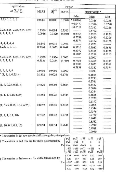
112

and SSVPC Charting Techniques for p = 5, n = 8 and a= 0.0027.

Eigenvalues _Power

ot L~1

L

1 MLRT

1s1112

SSVPf PR ()p()~Pn a

Max

2.25, 1, 1, 1, 1 _{0.0086 0.0100 0.0390}

_*

_0.0366

t 0.0470

:j: 0.0512

2.25, 2.25, 2.25, 2.25, 2.25 0.1356 0.4694 0.7560

---4, 1, 1, 1, 1 _{0.0946 0.0320 0.260.:1 0.2356}

0.2788 0.3174

4,4,4,4,4 _{0.8440 0.9232 0.9954}

---6.25, 1, 1, 1, 1 _{0.3064 0.0630 0.5444 0.5216}

0.6072

0.5806

6.25, 6.25, 6.25, 6.25, 6.25 0.9930 0.9974 1.0000

---9, 1, 1, 1, 1 0.5336 0.0844 0.7406 0.7456

0.7708 0.7838

9,9,9,9,9 0.9996 0.9990 1.0000

---b

0.1332 0.0026 0.1766

(1, 1, 1, 0.25, 4) _-----

----

---(1, 4, 0.25, 0.25, 4) 0.4620 0.0008 0.4624

---(1, 1, 1, 0.16, 6.25) 0.4358 0.0026 0.4414

---(1, 6.25, 0.16, 0.16, 6.25) 0.8692 0.0040 0.8156

---(1, 1, 1, 0.1, 10) 0.7622 0.0042 0.7398

---(1, 10, 0.1, 0.1, 10) 0.9894 0.0034 0.9644 _--

---

---*The entries in 1st row are for shifts along the pnnc1pal axes.

11./5 11./5 11./5

t The entries in 2nd row are for shifts determined by v.Ji _₁₁.Ji ₀

:j: The entries in 3rd row are for shifts determined by

r = 11./6 11 .J6 -21./6 11.ffi 11.ffi 11.ffi

1/ .fiiJ 11 .fiiJ 11 .fiiJ

0.88 -0.48 0.00

0.47 0.87 0.11

r=

-0.07 -0.13 0.52

-0.02 -0.03 0.85 0.00 0.00 -0.04

Med

0.0316

0.0376 0.0352 0.5792

0.2206

0.2450 0.2362

0.9926

0.5030

0.5418

0.5258 1.0000 0.7256

0.7626

0.7350 1.0000 0.1866

0.2990

0.2766

0.5422

0.6694 0.6244 0.4818 0.6226 0.6192 0.9006 0.9344 0.9396

0.7780

0.8642 0.8532 0.9910 0.9988 0.9930

11./5 11./5

0 0

0 0

-31.ffi 0

11.fiiJ -41.fiiJ

0.00 0.00

0.08 0.07

0.59 0.59

-0.34 -0.41 0.72 -0.69

Min 0.0268 0.0290

0.0226

---0.1926

0.2206

0.2176

---0.4636 0.4926 0.5110

---0.7188

0.7262

0.7174

Page 29

1 0.58 0.51 0.39 0.46

a _0.58

1 0.6 0.39 0.32 is used. I.o = 0.51 0.6 1 0.44 0.43

0.39 0.39 0.44 1 0.52 0.46 0.32 0.43 0.52 1

b The entries for the proposed technique are for the particular permutations of eigenvalues enclosed within

TABLE 6.

Pr(RL

~

k)

for a Change in

L.

after the rth Subgroup, by Proposed and MLRTECM Charting Techniques for p = 2, n = 3 and a= 0.0027.

I

' I

Eigenvalues I PROPOSED a

ot L.~1

L.

1 r k MLRTECM Max Min

4, 1 10 5 0.0110

*

0.1270 0.0675

t 0.1645 0.0680

:j: 0.1345 0.0615

10 0.0205 0.1750 0.0970

0.2195 0.0885

0.1860 0.1010

20 5 0.0125 0.2125 0.1255

0.2640 0.1365

0.2365 0.1205

10 0.0165 0.3000 0.2105

0.3165 0.1740

0.3205 0.1925

6.25, 1 10 5 0.0185 0.2785 0.1680

0.3265 0.1295

0.3205 0.1505

10 0.0375 0.3195 0.2180

0.3700 0.1505

0.3840 0.1765

20 5 0.0225 0.4515 0.3040

0.5015 0.2705

0.4725 0.2605

10 0.0495 0.5875 0.4230

0.6115 0.3405

0.6040 0.3680

9, 1 10 5 0~0360 0.4345 0.2840

0.4880 0.2015

0.5030 0.2370

10 0.0525 0.5080 0.3455

0.5660 0.2510

0.5185 0.2910

20 5 0.0485 0.6560 0.4785

i 0.6755 0.4100

0.6780 0.4625

10 0.0970 0.8050 0.6370

0.8045 0.5120

0.7965 0.5695

4, 4 10 5 0.0265

---

0.2285 ---10 0.0425 _--- 0.2760 ---20 5 0.0330 _------- 0.4205 ---10 0.0645 _--- 0.4890 ---6.25, 6.25 10 5 0.0675 _--- 0.4890 _______ ... _

10 0.1090 _--- 0.5115 ---20 5 0.0940 _----- 0.6935 ---10 0.1905 _--- 0.8035

---9, 9 10 5 0.1465 _--- 0.6965

---10 0.2270 _--- 0.7450 _----- ----20 5 0.2365 _--- 0.8770

---1 () () .d.1'J() _--- () Q~Q()

---*The entries in 1st row are for shifts along the principal axes.

t The entries in 2nd row are for shifts determined by r=(---0.9% 0.004

J·

---0.004 ---0.996

:j: The entries in 3rd row are for shifts determined by

r

= .

(

0.189 0.982] 0982 ---0.189

a .L,₀ =

( 1 0.5J

is used.

0.5 1

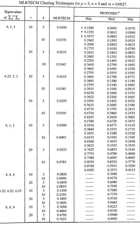
TABLE 7. Pr(RL~ k) for a Change in

L

after the rth Subgroup, by Proposed and

MLRTECM Charting Techniques for p = 3, n = 4 and a = 0.0027.

Eigenvalues _{PROPOSED a}

ot :L~1

:L1

r k MLRTECM Max Med Min

4, 1, 1 10 5 0.0100

_*

_{0.1385 0.0995 0.0370}

t 0.1535 0.0615 0.0560

:j: 0.1075 0.0850 0.0525 10 0.0170 _{0.1965 0.1395 0.0555} 0.2090 0.0810 0.0625 0.1735 0.1010 0.0790 20 5 0.0135 0.2425 0.1810 0.0855 0.2685 0.1215 0.0935 0.2205 0.1495 0.1015 10 0.0145 0.3410 0.2790 0.1045 0.3665 0.1695 0.1330 0.2795 0.1935 0.1395 6.25, 1, 1 10 5 0.0155 0.3405 0.2780 0.0775 0.3845 0.1380 0.1190 0.2795 0.2140 0.1065 10 0.0245 0.3915 0.3190 0.0915 0.4230 0.1660 0.1195 0.3625 0.2260 0.1605 20 5 0.0220 0.5505 0.2425 0.1925 0.5625 0.3085 0.2180 0.4710 0.3795 0.2415 10 0.0350 0.6710 0.5860 0.2335 0.6395 0.3650 0.3065

0.5780 0.4720 0.3475

9, 1, 1 10 5 0.0300 0.5520 0.4575 0.1110

0.5840 0.2515 0.1735

0.5055 0.3180 0.2320 10 0.0495 0.6135 0.5545 0.1505 0.6360 0.3055 0.2430 0.5625 0.3555 0.3195

20 5 0.0335 0.7625 0.6835 0.3145

0.7755 0.4780 0.4060 0.7380 0.6005 0.4445 10 0.0785 0.8530 0.8325 0.3770 0.8760 0.5915 0.5290 0.6505 0.5575 0.4115

4,4,4 10 5 0.0420

---

-

0.3940

---10 0.0690

---

0.4170

---20 5 0.0450

---

0.6040

---10 0.0810

---

0.7030

---6.25, 6.25, 6.25 10 5 0.1190 --- 0.7045

---10 0.2105

---

0.7570

---20 5 0.1895

---

0.9310

---10 0.3820

---

0.9685

---9,9,9 10 5 0.3090 --- 0.9215

---10 0.4460

---

0.9310

---20 5 0.4785

---

0.9940 ---10 0.7655

---

0.9995

Page 33

*The entries in 1st row are for shifts along the principal axes.

( 0.87

t The entries in 2nd row are for shifts determined by r

= _

036 0.34

0.23

044)

-0.31 0.88 .

-0.92 -0.19

( 0.85

:j: The entries in 3rd row are for shifts determined by r = 0.3 l -0.43

0.04

053)

-0.85 -0.43 .

-0.53 0.73

a [ 1

I.0 = o.75

0.45

0.45]

.

is used.

1 0.9

0.9 1

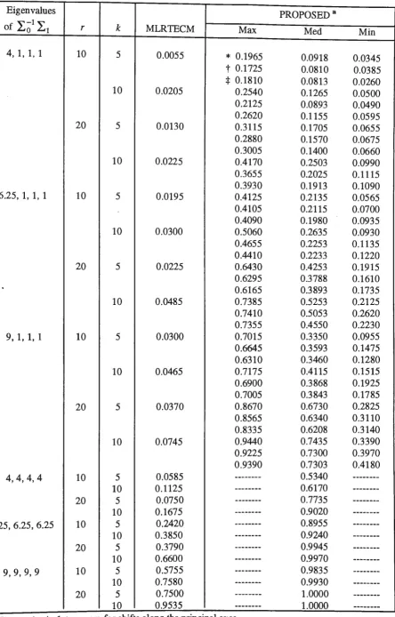
TABLE 8. Pr(RL::; k) for a Change in

L

after the rth Subgroup, by Proposed and

MLRTECM Charting Techniques for p = 4, n = 5 and a= 0.0027.

Eigenvalues _{PROPOSED a}

or

I.;

1

I.

₁ r k MLRTECM Max _{Med Min}

4, 1, 1, 1 10 5 0.0055

_*

_{0.1965 0.0918 0.0345}

t 0.1725 0.0810 0.0385 :j: 0.1810 _{0.0813 0.0260}

10 0.0205 0.2540 0.1265 0.0500

0.2125 0.0893 0.0490 0.2620 0.1155 0.0595

20 5 0.0130 0.3115 0.1705 0.0655

0.2880 0.1570 0.0675

0.3005 0.1400 0.0660

10 0.0225 0.4170 0.2503 0.0990

0.3655 0.2025 0.1115

0.3930 0.1913 0.1090

6.25, 1, 1, 1 10 5 0.0195 0.4125 0.2135 0.0565

0.4105 0.2115 0.0700

0.4090 0.1980 0.0935

10 0.0300 0.5060 0.2635 0.0930

0.4655 0.2253 0.1135

0.4410 0.2233 0.1220

20 5 0.0225 0.6430 0.4253 0.1915

0.6295 0.3788 0.1610 0.6165 0.3893 0.1735

10 0.0485 0.7385 0.5253 0.2125

0.7410 0.5053 0.2620

0.7355 0.4550 0.2230

9, 1, 1, 1 10 5 0.0300 0.7015 0.3350 0.0955

0.6645 0.3593 0.1475

0.6310 0.3460 0.1280

10 0.0465 0.7175 0.4115 0.1515

0.6900 0.3868 0.1925 0.7005 0.3843 0.1785

20 5 0.0370 0.8670 0.6730 0.2825

0.8565 0.6340 0.3110 0.8335 0.6208 0.3140

10 0.0745 0.9440 0.7435 0.3390

0.9225 0.7300 0.3970 0.9390 0.7303 0.4180

4,4,4,4 10 5 0.0585

---

0.5340

---10 0.1125

---

0.6170

---20 5 0.0750

---

0.7735

---10 0.1675

---

0.9020

---6.25, ---6.25, 6.25 10 5 0.2420

---

0.8955

---10 0.3850

---

0.9240

---20 5 0.3790

---

0.9945

---10 0.6600

---

0.9970

---9,9,9,9 10 5 0.5755

---

0.9835

---10 0.7580

---

0.9930

---20 5 0.7500

---

1.0000

---10 0.9535

---

1.0000

---*The entries in 1st row are for shifts along the pnnc1pal axes.

t The entries in 2nd row are for shifts determined by [ 0.96 -0.27

r= _0.04

-0.06

:j: The entries in 3rd row are for shifts determined by [0.96

' 0.28

r= _O.Ql

0.07

a [ I o.5 0.9 o.6] is used. :t = 0.5 1 0.2 0.7

0

0.9 0.2 0.4

0.6 0.7 0.4 1

0.11 0.11 -0.66

0.74 0.12

-0.23

0.62

-0.74

Page 35

0.26

0031

0.94 0.17 0.22 -0.72 0.02 -0.67

0.26

004)

-0.87 -0.33

-0.42 0.66

I

TABLE 9. Power Comparison of Proposed, IC and ISVPC Charting Technique for Shifts in the Form of

I.

₁ = A I, ₀.

Power

p n

a

A

Proposed IC ISVPC

3 4 0.0027 2.25 0.1688 0.1149 0.1334

4.00 0.6014 0.4666 0.5134

6.25 0.8664 0.7596 0.7965

0.01 2.25 0.2604 0.1995 0.2238

4.00 0.6818 0.5928 0.6342

6.25 0.8912 0.8404 0.8662

4 5 0.0027 2.25 0.2970 0.1669 0.2017

4.00 0.8300 0.6468 0.7097

6.25 0.9746 0.9127 0.9390

0.01 2.25 0.4050 0.2781 0.3216

4.00 0.8792 0.7672 0.8145

6.25 0.9822 0.9542 0.9686

5 8 0.0027 2.25 0.5792 0.3078 0.3877

4.00 0.9926 0.9036 0.9459

6.25 1.0000 0.9962 0.9986

0.01 2.25 0.7132 0.4648 0.5495

4.00 0.9938 0.9566 0.9772

Page 37

Appendices

A.1. The Distributional Properties of

w*

Depend on the Eigenvalues of L~t

Li

Lo~.

* .

Note that W may be wntten as

w*

= -

p(n -1)-(n -1)

lnlLo

i

s

Loi

I+

(n -

l)tr(

Loi s

Lo

~

)

s.t.

A1

0 0

rArT

=A=

diag(A-1, ... ,Ap

)=

0

A2

0 0 0 _AP

where A-1 ,. .. ,AP are the eigenvalues of A. Due to invariance w.r.t. any orthonormal

I

transformation (upon

Lo

2 _{X ),}

where

l'f

's are independently distributed as X~-i variables (see Theorem 3.3.8, p.82,

Srivastava et al.(1979)). Similarly,

tr(

L~t SL~!)

is distributed as

1 p

-~A..u.

(n-1)

fit

i i

where U i's are i.i.d X~-i variables. Combining these, the distribution of

w

*

therefore

depends on the combination of A-1, ... , AP . In addition, it is readily shown that the

I I

eigenvalues of

Lo

2

_Li

_Lo

2

characteristic equation. Note also that the result is not affected by the rotation of the

coordinate axes.

A.2. The Statistical Performance of

jsj

112 Chart Depends on the Product of the -.! --.!.

Eigenvalues of

Lo

2

L

1

Lo

2•

Note that the use of

jsj

112 charts with control limits of the form

kilLol

and k₂

1Lol

is

equivalent to charting and comparing the statistic

IL~!

S

Lo~

I

with the constants

ki

and

ki .

By using similar arguments to those in A.1, it is readily shown that the statistical

performance of this control technique depends on the product of the eigenvalues of

A.3. The Distributional Properties of The Sum of Standardized Variances of The _.! --.!.

Principal Components (SSVPC) Depend on The Eigenvalues of

Lo

2

L

1

Lo

2•

The sum of the standardized variances (multiplied by n - 1) of the principal components

is given by

t{<n-1>(

A~r

0

)s( A

0

lr

0

rJ

=tr[

(n -

l)A~tr

0

srJ A

0

~ J.

where A₀ and

rJ

denote respectively the diagonal matrix of the eigenvalues of

Lo

and

the matrix with the corresponding normalized eigenvectors. This statistic is invariant

I

w.r.t. any pxp orthonormal transformation (upon A₀2

r

0X). In particular, it is

Page 39

t{

(n

-I>rl(

A

0

~r

0

srJ

A-}

)r

₀

J

=

tr[(n

-1)(

r.;

A

0

~r

0

)s( rJ

A~!r

0

rJ

=

t{

(n

-1):~)

s(

~)

rJ

(see Johnson et al.(1988), p.51)

1

=

tr[<n-l)Loi

sL;t]

=

(n -

l)tr[ Loi

S

Loi

J.

·: Lo

2 _{is symmetric}

Note that this implies that the value of the plot statistic remains the same whether it is

computed from the principal components or any other set of linearly independent

combinations of the individual variables obtained in the above manner.

Now, let

r

be an orthogonal matrix such that

1 I

where

b

₁,b₂, ••• ,bP represent the eigenvalues of

Lo

2

L

1 L~2. Since

(n-l)tr[

Lo~ SL~t

J

=

(n-l)t{

r(

L

0

~ SL~!

)rT

J

where

r(

Loi

S

Loi

)rT -

WP (n

-1,

A)

when

I.= I.

1,

it is readily seen that the sum of

the standardized variances of the principal components is distributed as a linear

combination of p independent chi-square variables with n-1 degrees of freedom each and

A.4. Statistical Performance of MLRTECM Depends on the Eigenvalues of

I.~112 L1 I.;112

The MLRTECM criterion is W = -2lnA where

q 1

Ill 1

2 (n;-1) s(i)

A= i=1

I

s

pooled 1-t<ni+ ... +nq-q)

=C~-i-~"'--~~~~~~~

q 1<n1+ ... +nq-q)

L/ni -

l)S(i)

i=l

and C is a constant depending on the

ni 's

.

Due to invariance, A may be characterized

by

IT

q

I l.!.(n

·-1)

c

v.

2 _}

J

where

Vi -

WP ( n

i -1, I),

- WP(ni

-1, A),

j=l, ... ,r

j = r+ 1, ... ,q

r is the change point and A denotes a diagonal matrix containing the eigenvalues

"' "' of "'-112"" "'-112 Thus it is readily seen that the statistical performance of

/\;1, .. • 'l\;P ~o ~1 ~o · ,

Page 41

A.5. Scale Invariance of The Proposed Statistic (Known

I.

Case)

Let G =

diag(~

1

, . . .

,*)

be the diagonal matrix with ith element being the reciprocal of

the standard deviation of the ith variable. The sample covariance matrix computed from

the variables scaled to have unit variances (i.e the sample correlation matrix) is then

given by

s*

=GSGT

where d denotes the zero vector of (p-1) elements, S₂₂ is the sample covariance

matrix of the last (p-1) variables, and

ST = (R

12S1S2 R13S1S3 • •• R1PS1S P ). Similarly, the population correlation matrix is

where

L.22

represents the population covariance matrix of the last (p-1) variables and

matrix of the last (p-1) variables, given the first one, is

:-L.;2.1

= Dl'.22 DT - ( -1 Dl'.12)(1r1( -1

L.i2

DT)

0'1 ,..., 0'1

-= Dl'.22DT -DL.12(cri)-1 L.i2DT

,...,

-=D(

L22-L~2(cr:f

LJ2

)oT

= Dl'.22•1DT,

where _{L. 22•1} denotes the corresponding quantity calculated from the covariance matrix.

Note that the proposed charting variable is a function of, amongst others, the variance

ratio of the first variable and the Hotelling chi-square statistic based on the vector of

regression coefficients when each of the last (p-1) variables is regressed on the first

variable (1st off-diagonal vector divided by 1st diagonal element of the sample

covariance matrix). When calculated from s* and

L.

*, these are respectively

and

s*2 s2;cr2 s2

1 - 1 1 - 1

~*2 - 1 - 0'2