Application of modified Navier-Stokes equations to determine
the unsteady force effects of a heterogeneous liquid
František Pochylý 1, Roman Klas1 and Simona Fialová 1*
1Brno University of Technology, Faculty of Mechanical Engineering, Victor Kaplan Department of Fluids Engineering,
Technická 2896/2, 61669 Brno, Czech Republic
Abstract: The article is focused on calculating the force effects of a heterogeneous liquid on pipe walls. The solution is based on the concentration of solid particles. The base fluid is assumed to be incompressible. The solution will apply Euler-Lagrange's solution principle. Two tasks will be solved; with a rigid and a flexible tube wall. The solution will be carried out with non-stationary boundary conditions that were determined experimentally. Interaction of a heterogeneous fluid with a flexible wall assumes its deformation. The force effects will be solved by two methods; FSI simulation using ANSYS FEA solvers and CFD solvers ANSYS Fluent and using Navier-Stokes equations by direct integration through liquid volume. In this case, the unsteady term of the Navier-Stokes equations will be modified so that the Gauss Ostrogradsky theorem can be used to calculate the force. At the end, the force effects on the rigid and compliant wall will be compared with the unsteady turbulent flow of the heterogeneous liquid.
1
Introduction
In some model situations, including realistic cases, it is impossible to simplify the simulation of a liquid flow through an elastic medium (environment) by considering a homogeneous liquid[1][9]. As well as any solved three-dimensional area of approximately circular cross-section cannot be replaced by a smooth, perfectly circular tube[9]. These are two fundamental issues. The first is formed by the interaction of the liquid with the elastic wall itself [4], and the second represents the flow of heterogeneous liquids [2]. The FSI task is of course greatly dependent on the material and shape of the flow environment. In this respect, the addressed problem will be limited to a circular cross-section tube. Considering the heterogeneous fluid flow simulation, two main approaches can be chosen: Euler - Lagrange and Euler – Euler [5]. The Euler-Lagrange method is preferred in this work, with the heterogeneous liquid being the Lagrangian discrete phase model. The fluid phase is considered to be an incompressible continuum subject to the Navier-Stokes equations and the dispersed phase is formed by solid particles whose volume ratio does not exceed 10%. There is no further assumption of thermal or mass exchange between solid particles, and a simpler variant of a problem that does not involve
particle-particle interactions is considered. Depending on the means used to simulate the flow, it is possible to include or exclude these particle-particle interactions in the solution. In addition to a flexible material of the tube, rigid tubes were also considered to take into account the influence of the environment on the flow.
Considering the complexity of the problem, it is preferable to determine for example the force effect on the tube in a simpler way than the time-consuming FSI or CFD simulation. Definitive relationships suitable for the force analysis can be obtained from the Navier-Stokes equations and the continuity equation, as will be shown in the next part of this paper.
2
Analysis of forces for the
n-component system
The forces by which the liquid acts on the wall Γ, are generally determined from a stress tensor σij definition
[8] in relation to:
d n
Fi
ij j , (1)where n = (nj) is an external nominal vector oriented
Therefore, it is useful to express the power by using equations of equilibrium and the continuity equation.
The basic equations can be written in the form:
ij ij j i j i g x v v x v t
(2)
ii v x t
(3)
Assuming that ∂ρ/∂t = 0, equation (2) can be adapted to a suitable shape for using the Gauss-Ostrogradsky theorem. Suppose, therefore, that:
0
t
and therefore
0 i i v
x
(4)Considering this relationship, we can write with respect to equation (4):
i j ji x t v x
v
t
(5)By fitting into the continuity equation, we obtain a new equation of equilibrium:
0 ij l l ij j i i j j x g v v x v t
x
(6)From equation (6), the force that the liquid exerts on the rigid or the flexible wall can be determined, both at rest or in motion.
Let us consider the multiply contiguous region V, confined by wall Γ and surfaces S by which the liquid flows in or out of the region V. By integration of equation (6) through field V, we obtain a new relation for the force, which can be used for the analysis of the influence of inertial, volumetric and surface forces. For the ith-component of the force on surface Γ we can write a
relation:
S j ij j S l l ij j i i j i dS n d n x g v v x v t F
(7)Considering the definition equations for the concentration (8) and the velocity components (9), a more precise relationship for the force depending on the concentration (describes the effect of secondary discrete phase) can be determined. If holds
k kC (8)
and
k kj k kj
j v C
v
v
, (9)
then we determine the force from equation (10) as:
S j ij j S l l ij l k lj ki i k kj i dS n d n x g C C v v x C v t F
(10)The index k in the equation (10) denotes the individual phases of the heterogeneous liquid, and the terms of the equation can be divided according to these phases. From equation (10) it is also obvious that the force determines the conditions at the boundaries S unified with Γ. Thus, if the mixture is composed of two components ρ1 and ρ2, see equations (8) and (9), where ρ1
is the mass of the liquid relative to the unit volume of the mixture and ρ2 is the mass of the particles relative to the
unit volume of the mixture then, for example, with a fixed boundary Γ, v1i = 0 will hold for the liquid. We
assume that the liquid adheres to the surface of the tube. The term ∂v2i / ∂t ≠ 0 will reach high values, because the
particles impinge on the static wall of the tube and are reflected from it. This together with the equation (10), means that we will focuses on those terms of the equation in which the index k occurs. Then some terms can be reduced or a greater importance can be attributed to them. However, it practically means that the influence of the liquid as the primary phase 1 will be reduced as compared to the influence of the particles as a secondary phase 2. The particles present in the heterogeneous liquid can therefore significantly affect the strength of the rigid wall of the tube.
On the contrary, at a moving boundary Γ, which is an elastic wall of an elastic tube deformed by internal pressure, we generally apply v1≠0, v2i≠0, ∂v1i/∂t≠0 and
∂v2i/∂t≠0. However, if we look closer at the individual
terms, we find that the liquid 1 moves along the surface Γ along with this boundary and has the acceleration and velocity corresponding to the acceleration and velocity of that boundary. The greater the deformation of the tube wall, the more pronounced is the influence of the terms that take into account the phase of the heterogeneous liquid that belongs to the fluid phase, and for which k = 1. Meaning the terms v1i and ∂v1i/∂t. On the moving
surface, therefore, the dominant forces can be the p1 component, which is just the liquid. Conversely, the particle ∂v2i/∂t can be very small. The wall of the tube, to
some extent, yields to the particles by its own deformations. We also have to consider that v1≠0, of
course, on the moving surface from the point of view of the liquid, as well as the product (∂v1i/∂t) C1 in the
equation (10) predominates over the product (∂v2i / ∂t)
C2. The C2 concentration is less than or equal to 0.1, as it
was previously mentioned. All of this has the consequence that, in terms of the force effect, the influence of particles on the movable (elastic) wall may be suppressed, which is furthermore supported by their low concentration (C2). Therefore, the particles present in
impact on the magnitude of the force acting on the movable (elastic) wall of the tube. Conversely, in the case of a rigid tube, even lower concentrations of particles at different force effects, depending on their amount, will be reflected. This corresponds to the FSI and CFD results with a discrete phase simulation, as will be shown below.
3
Case geometry and CFD and FEM
software
The basic simulation tool was the ANSYS 18.2 commercial code with a structural FEA solver and CFS resolver ANSYS Fluent, which enables the interactions through the Discrete Element Method Collision Model. However, the above-described task was further simplified to the case where the wall of the tube was considered to be perfectly rigid, positioned horizontally, and particle-particle interactions did not occur. This had a reason so as to be able to analyse the force effect on the tube with respect to the description of the force based on the equilibrium and continuity equations.
Cylindrical geometry was further simplified to a one-quarter section of a circular cross-section. The reason for this step was to reduce the computational requirements that are significant with the FSI simulations. Of course, in the case of a tube, it is suggested to consider a two-dimensional task that would better fulfil the computational requirements, but the structural solver does not support a purely two-dimensional role. In line with the above, ANSYS DesignModeler and ANSYS Meshing were used to create 3D geometry of the tube and computer network. The basic information about the computer network, task settings and tube can be found in Tab. 1
Tab. 1 Calculation network, simulation conditions and tube parameters
Pipeline diameter 12.7 mm Width of the pipe
wall 1.6 mm
Observed total
length of the pipe 0.5 m, 0.7 m Pipeline material
(brand name) Tygon
Number of computational cells and calculated net type
FEM CFD 25 200
hexahedral hexahedral 156 030 and prismatic Material Hookean solid neo- liquid water Turbulence model
and near wall modeling
realizable k – ε enhanced wall treatment
Boundary conditions
Frictionless Fixed
Fluid solid interface
pressure inlet pressure outlet symmetry wall
Calculation mode incompressible unsteady, solid
unsteady, incompressible flow
As mentioned above, the FSI simulation, in addition to the fluid flow through the elastic medium, also endeavoured to include the influence of the discrete phase on the tube. In Tab. 2, the dispersed phase information is therefore provided. As has already been mentioned, particle-particle interactions do not occur, the particles do not aggregate or erode the surface of the tube. The rigid tube simulation in combination with the secondary phase was subject to the above set-up, but did not include a structural FEM solver.
Tab. 2 Discrete Phase Properties
Material anthracite
Diameter 1e-06 m
Diameter
Distribution uniform
Particle Type Inert
Injection Type surface, pressure inlet
Boundary Condition Type
wall reflect pressure
inlet escape
pressure outlet
Drag Law spherical
Input and output pressure sizes correspond to earlier tasks that have been addressed at the workplace in the framework of flexible tube testing. The readings of static pressures at the inlet and outlet of the tube are recorded in Fig. 1
Fig. 1 Inlet and outlet pressures in the elastic and rigid pipe
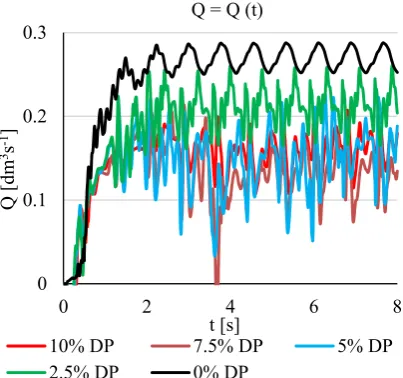
Fig. 2 shows the flow through a rigid tube with a different proportion of the dispersed phase determined at the centre of the tube. This gives us at least basic information about the flow.
Fig. 2 Flow in the rigid tube with different fraction of the dispersed phase
The flow in Fig. 2 fluctuates more than would be expected, and also changes more sharply than expected for individual dispersed phase (DP) fractions. This could be partly due to the simulated quarter of the tube. However, for comparison with the FSI, the role of the flexible tube required a quarter of the rigid tube to be
maintained. Control flow simulation in a circular cross section tube for 0% DP indicated that the flow amplitude was slightly smaller than shows Fig. 2, but the mean value is essentially the same.
Turbulence models also had a significant impact. Besides the model shown in Tab. 1, also tested were k - ω
SST and k-ε realizable with non-equilibrium wall functions [1], [6], [7]. However, the choice of the turbulence model was not unlimited due to the preservation of the identity of the computing network for CFD and FSI simulations. Therefore, a rigid circular tube with a fine computational network and a k-ω SST model was tested and based on this preference, the most suitable turbulence model using the wall functions and the coarse computation network was chosen. In fact, the flow simulation with the k-ω SST setting corresponded to a simple mathematical-physical model of the fluid flow in a rigid tube with 0% DP.
In the following Fig. 3, the magnitude of the radial forces acting on a quarter of the rigid tube is evaluated. We can say that the expected differences between the largest and the smallest ratio of the dispersed phase are well visible. In the remaining cases, the results are no longer so obvious and conclusive. This is of course also due to the fact that, at different times, a different amount of particles with a certain degree of independence on the dispersed phase and fluid phase share falls on the tube wall. The time scale is chosen so that it does not differ significantly from the simulation of the flexible tube. However, the beginning of the force recording with respect to Fig. 1 is not at t=0s. A steady section has been selected as far as possible. However, it would not be a problem to obtain a longer time recording of radial forces or flows.
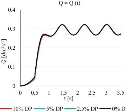
As in the case with a rigid tube, the FSI simulation of the flexible tube will first present the magnitude of the flows through the tubes defined in the center of the tube. The magnitude of the radial forces acting on the flexible tube is shown in Fig. 4. and Fig. 5. For time reasons in Fig. 4 and Fig. 5 simulation data for 7.5% DP are missing. However, due to the progress of the flows and forces, this does not represent a more fundamental problem.
Already the very low differences between the velocity values in the flexible tube (Figure 4) suggest that the differences between the forces will probably be small. We can say that the flow in the case of the flexible tube is primarily influenced by the movement of the flexible wall of the tube. Indeed, this also indicates the trend of radial forces in Fig. 5. The main force effect appears to be due to pressure pulsations in the tube and the effects of the dispersed phase are very low. By comparison with Fig. 3, it also indicates that the rigid tube forces have the character of sharp extremes in the form of minimums and maximums, which to a certain extent can be damped by the flexible tube. In view of the above analytical analysis of the force effect of the heterogeneous liquid on the 0
20 40 60 80 100
0 0.5 1 1.5 2 2.5 3 3.5
p s
tat
[k
Pa]
t [s] p stat = p stat (t)
pressure inlet pressure outlet
0 0.1 0.2 0.3
0 2 4 6 8
Q [dm
3s -1]
t [s] Q = Q (t)
10% DP 7.5% DP 5% DP
wall, it is also possible to confirm the conclusions regarding the effect of the solid particles. Its effect can be, according to Fig. 5, marked as minimal.
Fig. 3 Magnitude of radial forces acting on the rigid tube with different DP fraction
Fig. 4 Flows in the flexible tube with different fraction of DP
5
Conclusion
Flow rates through the quarter of a tube differ to a certain extent according to the used turbulence model. The differences are larger in this case than is the case with full 3D geometry. The test case is therefore more sensitive to the choice and setting of the physical model. Optimally, it would be understandable to implement the FSI simulation of the entire flexible tube. But the computational difficulty of such a task is untenable due to the acceptable time that the corresponding results
could be obtained in. Taking into account all the pitfalls, in this case, for the time being, the realization of the experiment seems to be the most advantageous way to obtain relatively fast data. Of course, if the experiment can be done. However, it is also worthwhile to look for other options in describing tube behavior, for example, based on analytical approaches.
Fig. 5 Magnitude of radial forces acting on the flexible tube with different DP fraction
If we evaluate the results of CFD and FSI simulations, we can say that in the case of CFD, the rigid tube simulation of the flow rate of the tubes or the amount of the dispersed phase corresponds to the radial force time recording. But for the individual quantities of the dispersed phase, the results are not entirely conclusive. However, there is a clear trend between the minimum and maximum fraction of the dispersed phase and the magnitude of the radial force. Deviations from the expected results are due to the irregular particle impact on the tube wall and the equally uneven effect of the particles on the current field in the tube. In the setting of this case, it is assumed that the particles are reflected from the wall of the tube and leave the system by the inlet and outlet cross-sections. It should also be taken into account that only a quarter of the tube has been simulated and full rotational symmetry is also assumed. However, the incident particles on the entire cylindrical wall of the tube can break this symmetry and the resulting radial force on the tube may not necessarily be completely zero.
As the computational mesh with the boundary conditions which in the simulation replace the liquid with or without a dispersed phase was identical for a rigid or flexible tube (CFD or FSI simulation), it cannot be said that distinctly different results in the radial force sizes acting on the tube are due to the considered quarter of the tube or computing network or boundary conditions. 0
200 400 600 800
0 0.5 1 1.5 2 2.5 3 3.5
Frad
[N]
t [s] Frad = Frad (t)
10% DP 7.5% DP 5% DP
2.5% DP 0% DP
0 0.1 0.2 0.3 0.4
0 0.5 1 1.5 2 2.5 3 3.5
Q [dm
3s -1]
t [s] Q = Q (t)
10% DP 5% DP 2.5% DP 0% DP
0 100 200 300 400 500
0 0.5 1 1.5 2 2.5 3 3.5
Frad
[N]
t [s] Frad = Frad (t)
In the FSI evaluation of the dispersed phase flexible tube, it appears on the contrary that the effects of the deformation of the tube due to the pressure field are more pronounced than the interactions of the secondary phase particles with the wall of the tube. The elastic tube also somewhat dampens the pulsation of the pressure and therefore the resulting radial force load on the tube slightly differs from the solid tube with the zero concentration of the secondary phase. It would be therefore worthwhile to test another flow model of a heterogeneous fluid based on the Euler - Euler approach, or to increase the existing dimensions of the dispersed phase particles and thus their weight. But the mass flow cannot be changed by the Euler-Lagrange method.
These conclusions fully correspond to the analytical analysis of the force on the tube and are in line with the definition of the forces that exert the load on the tube. If the wall of the tube is rigid, the velocity of the fluid on its wall is zero, and in the definition of force, apart from the pressure load, the effects of solid particles in the form of their pronounced local acceleration are applied. Particles are reflected from the rigid wall. Conversely, in the case of a flexible tube, the fluid velocity and its local acceleration on the wall are non-zero and correspond to wall movement. Furthermore, we must take into account the fact that the local acceleration of the liquid on the flexible wall significantly prevails over the local acceleration of the solid particles, which in combination with the low value of the solid particles C2 causes a dominant influence of the effects of the liquid. In a simplified way, it can also be said that the elastic wall impinges on the particles. Thus, the effect of solid particles on the movable wall in terms of force effect is practically not shown at least at concentrations up to 10% DP fraction to the fluid phase. Different results could also be obtained if the gravitational acceleration g, whether with a horizontal or a vertical tube, is considered.
However, it will be appropriate to supplement all of the findings with experimental measurements planned at a later stage, which should confirm or further refine the accuracy of the analytical analysis and FSI simulation with the discrete phase.
The force effect on the flow tube can be determined relatively smoothly for the smooth tube without time-consuming numerical FSI simulations, but it is more difficult to determine it for a tube whose surface is oval, corrugated or roughened. The same applies, of course, when a liquid is flowing through an area of other than a circular cross-section, which is also variable. Other complications are the flow itself, which may be in the stationary or non-stationary mode, and the above-mentioned homogeneous or heterogeneous base of the liquid. That is why the text describes the relations defining the magnitude of the force on the wall of the tube even for these general cases, considering the non-stationary flow. It is therefore possible to compare the
full numerical FSI simulation using ANSYS FEA solvers and CFS solvers ANSYS Fluent to validate the above mentioned relationships. It can further be assumed that the results obtained for simpler simulation tasks will be valid even for more complex areas of homogeneous or heterogeneous fluid flow through a rigid or flexible environment.
An experiment relating to the problem described was carried out on a flexible tube of circular cross section which was deformed by pressure pulsations. The deformation of the tube and the magnitude of the pressures were observed before and at the end of the measured area. Which were also verification values for all types of simulations of the described load of the tube by the flowing medium.
Grant Agency of the Czech Republic, within the project GA101/17-19444S and Technology Agency of the Czech Republic, within the project TE 02000232 are gratefully acknowledged for support of this work.
References
[1] Embid, P. and Baer, M.R.: Mathematical analysis of a two phase continuum mixture theory, 1992, Continuum mechanics and thermomechanics, Vol. 4, pp. 279-312
[2] Prosperetti, A. and Tryggvason, G.: Computational methods for multiphase flow. Cambridge University Press, 2009. ISBN 978-0-521-13861-1 [3] Brennenm C.E.: Fundamentals of multiphase flows.
Cambridge University Press, 2005. ISBN 0521 848040
[4] Giannopapa, C.G.: Fluid structure interaction in flexible vessels. (CASA-report; Vol. 0622). 2006 Technische Universiteit Eindhoven.
[5] Ballard, D.H.: An introduction to natural computation, MIT press, 1999, ISBN-13: 978- [6] Mohammadi, B., & Pironneau, O. (1993). Analysis
of the K-epsilon turbulence model. France: Editions MASSON.
[7] Mansour, N. N.; Kim, J.; Moin, P. Near-wall k-epsilon turbulence modeling, 6th Symposium on Turbulent Shear Flows, France, Proceedings (A88-38951 15-34). University Park, PA, Pennsylvania (1987), p. 17-4-1 to 17-4-6.
[8] Fridtjov Irgens: Continuum Mechanics, 2008 Springer. ISBN 3-540-74297-2