Constructing confidence intervals for QTL location.

Copyright 0 1994 by the Genetics Society of America

Constructing Confidence Intervals

for QTL Location

B. Mangin, B. Goffinet

and

A. Rebai

Znstitut National de la Recherche Agronomique, Station de Biomitrie et d ’Intelligence Artaficielle, 31326 Castanet-Tolosan Cedex, France

Manuscript received December 6, 1993 Accepted for publication August 3, 1994

ABSTRACT

We describe a method for constructing the confidence interval of the QTL location parameter. This method is developed in the local asymptotic framework, leading to a linear model at each position of the

putative QTL. The idea is to construct a likelihood ratio test, using statistics whose asymptotic distribution does not depend on the nuisance parameters and in particular on the effect of the QTL. We show

theoretical properties of the confidence interval built with this test, and compare it with the classical confidence interval using simulations. We show in particular, that our confidence interval has the correct probability of containing the true map location of the QTL, for almost all QTLs, whereas the classical confidence interval can be very biased for QTLs having small effect.

F

OLLOWING SAX (1923), many methods have been developed in the literature for detecting quantita- tive trait loci (QTL) using marker information. Estimat- ing QTL map location is possible using “interval m a p ping” procedures based on maximum likelihood estimation (LANDER and BOTSTEIN 1989) or on linearized version of maximum likelihood (KNNP et al. 1990; HALEYand KNOTT 1992). As pointed out by DARVASI et al.

(1993), a very important quantity is the confidence in- terval of the QTL position on the chromosome.

CONNEALLY et al. (1985), in the field of linkage analy- sis, and LANDER and BOTSTEIN (1989) proposed the use of a confidence interval based on limiting

x2

distribution of the likelihood ratio test between two positions. This idea leads to a very simple construction of the confi- dence interval: take the maximum value of the LOD score, substract c, and the locations corresponding to this value of the LOD score are the extremes of the con- fidence interval (at 96.8% when using c = 1).

As

we will see, simulations show that the

‘

x

approxi- mation is not correct for QTLs having small effect, and therefore that the corresponding confidence intervals are biased, e.g., the probability of the QTL being in an interval is less than the nominal level. The reason for this is that the regularity conditions for the convergence of the likelihood ratio test toward a

2

distribution are not fulfilled for QTLs having small effect.

In this report, we will study the asymptotic properties of the likelihood ratio test for QTLs having small effect and construct a new test and therefore a new unbiased confidence interval.

MODEL AND CLASSICAL CONFIDENCE INTERVAL We consider a backcross sample of size n. Consider a QTL present at the position d on a chromosome of length L. The trait value has a normal distribution with

Genetics 1 3 8 1301-1308 (December, 1994)

means p A and pB for the two QTL genotypes present in the backcross population and the same variance

4,

for both genotypes. We will use a = p A - kB and p = ( k A

+

pB)/2. For each individual k = 1,

. .

.

, n, we score the phenotypic value of the trait

y k

and a set o f j = 1,

. . .

,

Jmarkers with the information Mj,k that takes the values

A or B depending on the allele of the marker. The vector of phenotypic observation will be denoted by Y, and the vector of all marker information by At.

The likelihood of Y, conditional on the marker in- formation is LA( Y, a, k , r?, d). Its complete expression is given by LANDER and BOTSTEIN (1989)

LA ( Y , a, k , u2,

4

=

n

LG&(’9 d)’$(l)

+

(l - d)llk(O))

k

where G,( k, d ) is the probability for individual k to have genotype A at position d, conditional on the marker information A; Zk(x) = +( yk - p

-

xu, r ? ) , for x equal 0 or 1, is the probability density function for the normal distribution with mean 0 and variance

4.

In the follow- ing, we assume no interference in recombination events and therefore use Haldane’s map function. This func- tion associates distance d with recombination probabil- ity r ( d ) = 0.5(1 - exp(-2d)).

A confidence interval can be built as follows

( CONNEALLY et al. 1985): at each point do along the chro- mosome, perform the likelihood ratio test

~ 4 )

= 2 1n S U P , ~ , ~ ~ L ~ ( Y , a, P, u2,

4)

~ u p ~ , ~ & ( Y , a = 0, CL, u2,

4)

*

Note that the LOD score test is essentially the same test

B. Mangin, B. Gofinet and A. Rebai

3 4

0 1 2

Value of parameter a

We can now calculate the test T ( do)

q4)

= sup

[ a d ) ]

- R ( 4 ) d

SUpGp,u~,dL&(Y,

a>

P> u',

d)

s u p G + , u ~ ~ ~ ( y , a, p9 (+*1

4)

*

= 2 In

Considering that T ( do) follows a

x'

distribution with one degree of freedom under the null hypothesis, that is do is the correct position, the (1 - a ) confidence in- terval is: [ dinf, dsup], where dinf ( &,) is the smallest (the greatest) value of do such that T ( do) is smaller than

x;,a;

is the a quantile of a

x'

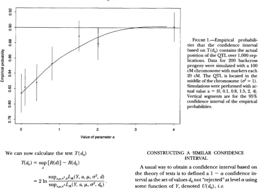
with 1 d.f.

The theory underlying this confidence interval is cor- rect for any non-null finite value of a and an infinite number n of individuals. To investigate the quality of this confidence interval, we perform simulations for some a values with n = 2 0 0 , 4 = 1 and a chromosome of length 100 centiMorgan (cM) having markers each 20 cM (Figure 1) and 5 cM (Figure 2). The QTL is located in the middle of the chromosome in the first case, and at d = 47.5 cM in the second case. It appears that the confidence interval is unbiased for large values of a but can be very biased for small values of a, particularly in the case of a dense map.

The reason for this is that for small value of a, the likelihood ratio test T ( d ) does not follow a

x'

distribu- tion, when the QTL is located at d. Table 1 shows that the quantiles of the distribution of T ( d ) are different from those of a

x*.

The difference depends on the

a

values and is quite large when a is small.

The following section gives a theoretical framework to deal with these small values of a.

FIGURE 1 .-Empirical probabili- ties that the confidence interval based on T(d,) contains the actual position of the QTL over 1,000 r e p lications. Data for 200 backcross progeny were simulated with a 100 cM chromosome with markers each 20 cM. The QTL. is located in the middle of the chromosome

( 4

= 1). Simulations were performed with ac- tual value a = (0, 0.1, 0.8, 1.5, 2, 4). Vertical segments are for the 95% confidence interval of the empirical probabilities.

CONSTRUCTING A SIMILAR CONFIDENCE INTERVAL

A usual way to obtain a confidence interval based on the theory of tests is to defined a 1 - a confidence in- terval as the set ofvalues do not "rejected" at level

a

using some function of Y, denoted U( do), i.e.

(4;

u(4J

5

dd,,)}

P [ U ( 4

>

C J 4 ) l

= a* with

In models where there are nuisance parameters, the central requirement for this procedure is to be similar for all the nuisance parameters, i.e., the probability of U( d,,) being greater than c( d,,) equals a for all the nuisance pa- rameters. That is not the case for the classical procedure.

Basic ideas: To obtain a similar procedure for all the nuisance parameters ( p ,

4,

a ) , we propose to use a similar test, as described by Cox and HINKLEY (1974). The basic idea for similarity is to find statistics whose distribution does not depend on the parameter a under the null hy- pothesis: the QTL is located at

4.

Suppose that, under the null hypothesis,

Go

is a s d c i e n t statistic for the parameter a then a good

way

to obtain similar procedure is to work with the conditional distribution of Y given

zq

Confidence Intervals for QTL 1303

t

I

0 1 2

Value of parameter a

TABLE 1

Empirical quantiles and their 95% confidence interval for the

distribution of T(do) over 1,000 replications

Quantile

10% 5%

X: 2.71 3.84

a = 0.1

'

49 4.89 5,69 3.34 3.75 .109

a = 0.8

5 1 8 5.96 6 , 4 2

'." 4.51 5,18

a = 0.4

5.96 6.36 7,42 '." 5.07 5,42

In each cell, the number in the middle is the empirical quantile and the italic numbers in the corners are the lower and upper bounds of a 95% confidence interval for the quantile.

Data for 200 backcross progeny where simulated with a lOOcM chromosome with markers each 5 cM. The QTL is located at a dis- tance of 47.5 cM from one end of the chromosome (d = 1).

the maximum likelihood ratio test for QTL detection converges to 1 (Table 2).

Formally, in the local asymptotic framework, as n + 00,

a is assumed to tend to 0 in such a way that a f i converges to a finite constant 6 (Cox and HWKLEY 1974, p.317). FEIN- GOLD et al. (1993) used the same asymptotic framework.

In this framework, T ( do) is not asymptotically distrib- uted as a

2

under the null hypothesis. This is because the information matrix is not positive-definite for a = 0, and therefore the classical Taylor expansions cannot be made in the neighborhood of a = 0. In particular, the parameter d cannot be estimated consistently for a = 6/<n, i. e . , the maximum likelihood estimator

d

of d does not converge toward d when the number of ob- servations tends to infinity. This can be easily seen in a

FIGURE 2.-Empirical probabili- ties that the confidence interval based on T ( do) contains the actual position of the QTL over 1,000 r e p lications. Data for 200 backcross progeny were simulated with a 100 cM chromosome with markers each 5 cM. The QTL is located at a dis- tance of 47.5 cM from one end of

the chromosome

( 4

= 1 ) . Simula- tions were performed with actual value a = {0,0.1,0.8,1.5,2,4}.Vertical segments are for the 95% confi- dence interval of the empirical probabilities.

3 4

TABLE 2

Empirical power (in %) of interval mapping for QTL detection

over 1,000 replications

n

200 800

5% quantile 1% quantile 5% quantile 1% quantile at density at density at density at density

(cM): (cM): (cM): (cM):

a 20 5 20 5 20 20

0.1 8.5 9.0 1.0 1.2 18.2 4.2 0.4 59.8 64.0 28.4 30.0 99.3 95.2 0.8 99.3 99.9 95.2 98.5 100.0 100.0

The QTL is located in the middle of the chromosome for a marker density of 20 cM and at a distance of 47.5 cM from one end of the chromosome for a marker density of 5 cM

(4

= 1).

simple situation with only two markers that is treated in detail in the following section.

The new test: Working in the local asymptotic frame- work, asymptotically sufficient statistics can be found for the parameters a,

w,

d,

d. These are

p,

the global mean,

(i2,

the classical estimator of the variance, and the mean class difference at each marker Sj; j = 1,

. . .

,

J

1304 B. Mangin, B. Goffhet and A. Rebai

regression estimators in the linearised model of KNAPP

et al. (1990) and HALEY and

&om

(1992) are asymp- totically equivalent ( e . g . , convergent in probability).

Consider now

z4

the maximum likelihood estimator of a if the QTL is located at do and Z( do) the vector of components

Z,(

do); j = 1,

. . .

,

J - 1 defined by:

where rj, do denotes the probability of recombination between the marker

j

and a QTL located at do.

Proposition 1 (proven in APPENDIX [All) shows that Z ( do) is asymptotically a similar statistic for all the nui- sance parameter when the QTL is supposed to be lo- cated at do.

Proposition 1. Under the null hypothesis-the QTL is

located at do-we get:

where the matrix V depends only on the length of the chromosome and the position of the makers.

Proposition 2 (proven in APPENDIX

[MI)

gives the as- ymptotic distribution of Z ( d o ) when the QTL is sup- posed to be located at d.

Proposition 2. Under the alternative hypothesis-the QTL is located at d-, we get:

where the vector X(d, d,,) depends only on the length of the chromosome, the position of the makers, d and d,.

Using the asymptotic distribution of Z ( d o ) we can build a maximum likelihood ratio test T z ( d o ) ,

where L a ( * ) means that the likelihood is calculated with the asymptotic distribution of Z ( d o ) and

6

= 6 / a .

This gives:

where:

W ( d ,

4,)

= X(d,

4 ) ' V - ' q 4 )

and Var,(.) denotes the variance for the asymptotic dis- tribution of Z ( d o ) .

The algebric expression of T z ( d o ) is given in the

APPENDIX [ M I .

THRESHOLD CALCULATIONS

To be able to use the confidence interval built with T z ( d o ) , we need the asymptotic distribution of this sta-

tistic under the hypothesis that the QTL is located at do. This distribution does not depend on the parameters 6,

4

and p, but may depend on the length of the chro- mosome, the number and the position of the markers and the position do.

The case with only two markers: In this situation, the statistic W ( d , d o ) does not depend on d. So, the asymp- totic distribution of Tz( do) under the null hypothesis is a

x:.

Looking at the algebric expression of W ( d , d o ) , given in the APPENDIX [A3], we see that:

1

where

p

is the recombination probability between the two markers and r ( d o ) the recombination probability between the QTL and the first marker.

We get as a 1 - a confidence interval, the set of points:

The end points of the confidence region for the parameter

( 1 -

24

4 )

) appear to be the solution of a quadratic func- tion. In particular, the confidence region is not symmetric around the maximum likelihood estimator of d. Note that we observe here the same type of result as RELLER (1954) with the confidence interval of the ratio of two random variables.

Another feature of the case with only two markers is the fact that the classical confidence interval and the new con- fidence interval could be the same. APPENDIX [A41 explains this particularity and the non-consistency of the likelihood estimator of d in the local asymptotic framework.

The case with more than 2 markers: In this case, the asymptotic distribution of T z ( d o ) is the distribution of the supremum of a

x:

process with a covariance function depending on do. As it is difficult to obtain this distri- bution using analytical arguments, we propose to use simulations. These simulations are made using the as- ymptotic distributions of the Sj for

j

= 1,

. . .

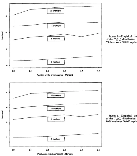
, J.

Figures 3 and 4 show the c,(

4)

threshold functions of this distribution for the 5 and 10% levels and for diEerent numbers of markers equally spaced along the chromo- some. In these cases, the threshold function c,( $) is sym-

metric around the middle of the chromosome so we give this function for half of the chromosome.

RESULTS AND DISCUSSION

Confidence Intervals for QTL 1305

- 1 ~~

0.0 0.1 0.2 0.3 0.4 0.5

Position on the chromosome (Morgan)

-

1

6 markers

1

FIGURE 3.-Empirical threshold of the T,(d,) distribution for the 5% level over 50,000 replications.

FIGURE 4.-Empirical threshold

of the Tz(do) distribution for the 10% level over 50,000 replications.

0.0 0. I 0.2 0.3 0.4 0.5

Position on the chromosome (Morgan)

Table

3

gives the empirical probability for the interval to contain the actual position of the QTL. Simulations are made with a chromosome of

1

Morgan, with markers at each

20

or

5

cM with n =

200

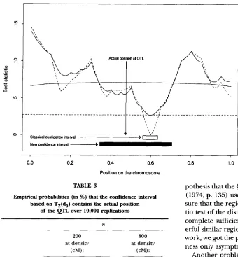
or n = 800. It appears that the confidence interval is unbiased for all values of a that have been used.

We show in detail a simulated example in Figure

5.

This simulation has been performed with n =

200,

a = 0 . 4 , d

=

1

and a marker at each 5 cM. The dashed line represents T( d ) and the classical confidence interval is the set of the

points behind the threshold

2.71.

The full line represents

T,(

d ) and the threshold is that shown in Figure

4.

In this case, the actual position of the

QTL,

shown with an mow on Figure 5, is not in the classical confidence interval but is in the new one. We obtain this type of result in about

20%

of the replications.

B. Mangin, B. Goffinet and A. Rebai

0.0 0.2 0.4 0.6

Position on the chromosome

TABLE 3

Empirical probabilities (in %) that the Confidence interval

based on TZ(cb) contains the actual position

of the QTL over 10,000 replications

n

200 800

at density at density (cM) : (cM):

a 20 5 20

0.1 90.0 90.3 90.6

0.5 89.5 89.6 89.9

1 89.6 89.8 89.9

2 90.4 89.8 89.4

4 89.7 89.6 89.8

The QTL is located in the middle of the chromosome for a marker density of 20 cM and at a distance of 47.5 cM from one end of the chromosome for a marker density of 5 cM (0' = 1 ) . All the empirical probabilities are in the 99% confidence region of 0.9.

position do in a specific situation must be found. In Figures

3 and 4, we give the threshold function for some situations. For other situations, far from the equally spaced number of markers studied, specific simulations should be per- formed. Even if the use of Tz(

4)

seems to be more com- plicated than the use of T(

4 ) ,

it must be preferred because it guarantees an unbiased confidence interval. Moreover, a correct threshold for T(

4)

cannot be obtained because it depends on the value of the unknown parameter a.

In the general case, we have no information on the power of the test Tz( do) and therefore on the length of the new interval. However, we worked with asymptotic sufficient statistics and can argue for completion of

{p,

2,

;;$

in the local asymptotic framework under the null hypothesis. Then in this framework, Z ( d o ) contains all the informations coming from Y, concerning d and not depending on the nuisance parameters under the hy-

FIGURE 5.-Confidence intervals for the position of the QTL built respectively on T ( d o ) and T,( do).

Data for 200 backcross progeny were simulated with a 100 cM chro- mosome with markers each 5 cM

( 4

= 1). The actual position of the QTL is pointed with the vertical ar- row and its actual value is a = 0.4. The full line is T,(d,) and the

threshold is that shown in Figure 4. The dash line is T ( do) and the con- fidence interval is the set of points below the threshold 2.71.

pothesis that the QTL is at position do. COX and HINKLEY

(1974,

p.

135) used the argument of completion to en- sure that the region constructed with the likelihood ra- tio test of the distribution of the data conditioned on a complete sufficient statistic is the uniformly most pow- erful similar region. The main difference is that, in our work, we got the properties of sufficiency and complete- ness only asymptotically and locally.

Another problem is to calculate the probability that the confidence interval contains the actual position o f the QTL, conditional on to the fact that the LOD score test is greater than its threshold.

FEINGOLD et al. (1993), in the framework of identity by descent mapping, gave approximate confidence regions for gene position based on sophisticated theoretical de- velopments about point processes in the case of an ide- ally dense map. Their approach could be adapted in our situation and would give interesting results for this kind of map.

An interesting use o f these confidence intervals is when one wants to test the consistency of a QTL over different environments or crosses. For instance, suppose a QTL was detected in some environment with a specific effect and position on the chromosome. A QTL in the same region of the chromosome was also detected in another environment but with different genetic effect (e.g., PATTERSON et al. 1991). Some developments around our method could permit a test of whether the locations of the QTLs in both environments are the same.

Confidence Intervals for QTL 1307

Thanks are due to the referees whose comments clarified many issues and led to a better presentation.

LITERATURE CITED

CONNEALLY, P. M., J. H. EDWARDS, K. K. KIDD, J. M. LALOUEL, N. E. MORTON et al., 1985 Reports of the committee methods of linkage analysis and reporting. Cytogent. Cell Genet. 40:

Cox, D. R., AND D. V. HINKLEY, 1974 Theoretical Statistics. Chapman & Hall, London.

DARVASI, A,, A. WEINREB, V. MINKE, J. I. WELLERAND M. SOLLER, 1993 De- tecting marker QTL gene effect and map location using a satu- rated genetic map. Genetics 134 943-951.

FEINGOLD, E., P. 0. BROWN AND D. SEGMLIND, 1993 Gaussian mod- els for genetic linkage analysis using complete high-resolution maps of identity by descent. Am. J. Hum. Genet 5 3 234-251.

FIELLER, E. C., 1954 Some problems in interval estimation. J. R. Stat.

HALEY, C. S., AND S. A. h o r n , 1992 A simple regression method for

Heredity 69: 315-324.

mapping quantitative trait loci by using molecular markers.

KNAPP, S. J., W. C. BRIDGES AND D. BIRKES, 1990 Mapping quantitative trait loci using molecular marker linkage maps. Theor. Appl. Genet. 79: 583-592.

LANDER, E. S., AND D. BOTSTEIN, 1989 Mapping Mendelian factors un-

derlying quantitative traits using RFLP linkage maps. Genetics

121: 185-199.

MELCHINGER, A. E., 1990 Use of molecular markers in breeding for oligogenic disease resistance. Plant Breed. 1 0 4 1-19.

PATERSON, A. H., S. DAMON, J. D. HEWITT, D. ZAMIR, H. D. RABINIWITCH

et al., 1991 Mendelian factors underlying quantitative traits in

ments. Genetics 127: 181-197.

tomato: comparison across species, generations and environ-

REBA~, A,, B. GOFFINET AND B. MANGIN, 1994 Comparing power of dif- ferent methods for QTL detection. Biometrics (in press).

SAX, K, 1923 The association of sizes differences with seed coat pattern and pigmentation in Phaseolus v u l g a r u s . Genetics 8: 552-560.

356-359.

soc. B 16: 175-185.

Communicating editor: B. S. WEIR

APPENDIX

[All In the local asymptotic framework, the maximum likelihood estimators are asymptotically equivalent to the regression estimators using the linearized model:

y k =

+

aGA4(b

d)

+

‘k

where the ek are independent and identically distributed as

normal with mean 0 and variance c? (REM et al. 1994). Using the linearized model, it is simple to see that $,

and the Si for j = 1,

.

. .

,

J are asymptotic sufficient

In the following, we will use that l[,,,=Al/n and

For the null hypothesis-the QTL is located at do- statistics for p, a‘, S and d.

l,y,h=,/n both converge in probability to

X.

we get:

where id, is the left marker of the interval where the QTL is located,

T , ~

( r J is the recombination rate be-

tween the QTL and the marker j (between the markers

i

and j) and xa,b = (1 - 2 r 0 J .

As

62

converge in probability to

4,

it is sufficient to study the distribution of the statistics

4

for j = 1,

. . .

,

J i n the linearized model, to get the asymptotic dis-

tribution of

(fizd,

a d , ) ) .

In the linearised model, S , the vector of components

Sj, is multinormal. This implies that

&,

and Z ( 4 ) are asymptotically and locally multinormal.

Under the null hypothesis:

E(%)

= [(l - 2?j4)/2]S.

So we get:

my4))

= 0

Cov(S,,

%+J

= a 2 ( P r ( 4 . = A, M,+, = A )

+

Pr(Mj = B, Mj+, = B ) - Pr(Mj = A, Mj+l = B )

-

Pr (M, = B, Mj+l = A ) )

= a2(1 - 2?jj+J

So, the matrix V depends only on the length of the chromosome and the location of the markers.

Besides, given three points on the genome, denoted

a, b, c, located in term of probability of recombination

by r,,,, rb,c and ra,c, if b is located between a and c we get, assuming no interference in recombination events:

‘a,r = xo,bxb,c (3)

Using ( 3) , we get:

COV(Z@ Z,(&)) = 0

[ A 2 1

To obtain the asymptotic distribution of Z( d o ) , we study the distribution of

S

in the linearised model under the alternative hypothesis-the QTL is located at d-.

E(%)

--

[(l - 27,,)/2]6

We then get:

E(z4)

2.X ( d t

4)(S/a)

where the j t h component of the vector X ( d ,

4)

is:

X(d,

4)j

= (Xj,&,d,

-

X j + * , d / X j + 1 , $ ) (4)

The same arguments than in APPENDIX

[All

provides for Z(do) an asymptotic normal distribution with vari- ance V.

[ A 3 1

The expression of W( d,do) is:

% - I

w ( d 4 )

= ai&&,b($)

+

aid<d,(&) i-

x

q(4)

for i d <

‘4,

,=“+I

W d

4)

=

4&4)

for id = i4

W ( d ,

4 )

= ai,

4&(4)

+

aiid.q4)

+

E

g(&)

for id > id,

“-1

1308 B. Mangin, B. Gofinet and A. Rebai

with

Using that Vis a diagonal matrix with diagonal ele- ment equal to:

1 x,,,+ 1 1

2

v..

=

-

-

+-

the algebric expression of T,(do) is easily found.

J J x;, xj,45+1,& ' ; + I , ,

Details of calculations: Using

(2)

we get:

v .

=-- 5 , j + I I+ 1

X j , 4 5 + L 4 x j , 4 x j + l + 1 . 4

-

X j + l , j + I x j + l , j + l + l 1.J+I

+

5 + 1 , , X j + r , x j + l , , X j + I + l , &

Now, using (3) and the

QLT

position under the null

Suppose that id

<

zdo, we obtain using (2), (3) and

(4)

: hypothesis, give y , j + . l =

0

for 1 > 0.

4)j

[A41

In the local asymptotic framework, consider

the asymptotic distribution, under the null hypoth- esis, of the vector

S,

which elements are SI and

S,

divided by

m:

with

w =

(

x:,z x ; z )

where x i , j is defined in APPENDIX [ A l l .

Maximum

likelihood estimator for the parameter

d:

Using the linearised model and the vector U( d ) , we found that an asymptotic equivalent statistic of the maximum likelihood estimator for = (1 - 2r(d))2 is:

j < id

j = id

i d < j < id,

j = i,

i4

<

j .

Because the test is invariant by scale, the constant xd, do

can be left and we find the expression given for W( d, do) in the case id

<

i,.

For id = i,, we get:

And for id

>

i,:

X ( 4

a i

This estimator does not converge towards (1 -

2r(

d ) ) 2 . Therefore, the maximum likelihood estimator for the parameter d does not converge toward d.

Asymptotic equivalence between Tz(do) and Tz(do):

Denote PG:, the projector onto the linear space gen- erated by U( do) for the W" norm, P:I(i, the projector onto the orthogonal of the space for the W" norm

and

11.

.

.]I;-,

the square of the W" norm.

When only 2 markers are present on the chromo- some, it can be proved that T( do) and T,( do) are equiva-lent when

The probability of this event is not null, because the region covered by {& U( d ) } and the vector S' are both in a two dimensional space.