TFHE: Fast Fully Homomorphic Encryption
over the Torus
?Ilaria Chillotti1, Nicolas Gama3,2, Mariya Georgieva4,3, and Malika Izabach`ene5
1 imec-COSIC, KU Leuven,
Kasteelpark Arenberg 10, Bus 2452, B-3001 Leuven-Heverlee, Belgium [email protected]
2
Laboratoire de Math´ematiques de Versailles, UVSQ, CNRS, Universit´e Paris-Saclay, 78035 Versailles, France
3
Inpher, Lausanne, Switzerland [email protected], [email protected]
4 EPFL, Route Cantonal, CH-1015 Lausanne, Switzerland 5
CEA, LIST, Point Courrier 172, 91191 Gif-sur-Yvette Cedex, France [email protected]
Abstract. This work describes a fast fully homomorphic encryption scheme over the torus (TFHE), that revisits, generalizes and improves the fully homomorphic encryption (FHE) based on GSW and its ring vari-ants. The simplest FHE schemes consist in bootstrapped binary gates. In this gate bootstrapping mode, we show that the scheme FHEW of [29] can be expressed only in terms of external product between a GSW and a LWE ciphertext. As a consequence of this result and of other optimiza-tions, we decrease the running time of their bootstrapping from 690ms
to 13mssingle core, using 16MB bootstrapping key instead of 1GB, and preserving the security parameter. In leveled homomorphic mode, we propose two methods to manipulate packed data, in order to decrease the ciphertext expansion and to optimize the evaluation of look-up tables and arbitrary functions in RingGSW based homomorphic schemes. We also extend the automata logic, introduced in [31], to the efficient lev-eled evaluation of weighted automata, and present a new homomorphic counter called TBSR, that supports all the elementary operations that occur in a multiplication. These improvements speed-up the evaluation of most arithmetic functions in a packed leveled mode, with a noise over-head that remains additive. We finally present a new circuit bootstrap-ping that convertsLWEciphertexts into low-noise RingGSW ciphertexts in just 137ms, which makes the leveled mode of TFHE composable, and which is fast enough to speed-up arithmetic functions, compared to the gate bootstrapping approach.
Finally, we provide an alternative practical analysis of LWE based schemes, which directly relates the security parameter to the error rate
?This work was done while I. Chillotti was a PhD student in the Laboratoire de
of LWE and the entropy of the LWE secret key, and we propose concrete parameter sets and timing comparison for all our constructions.
Keywords: Fully Homomorphic Encryption, Bootstrapping, Lattices, LWE, GSW, Boolean circuit, deterministic automata.
1
Introduction
This paper is the complete and extended version of the two papers [22] and [24] published by the same authors at Asiacrypt 2016 and Asiacrypt 2017, respec-tively. It unifies the work presented in both, completes the proofs, adds some further explanations of the results and experimentally validates the Gaussian output noise heuristic.
Since Gentry introduced in 2009 [33] the concept of bootstrapping, and proved that fully homomorphic encryption was achievable in polynomial time, many constructions have appeared, involving new mathematical and algorith-mic concepts, improving efficiency and memory requirements. Nowadays, the most promising constructions [52, 12, 34] rely on two lattice-based problems: approximate-GCD, presented by Howgrave-Graham in 2001 [38], and Learning With Errors (LWE), presented by Regev in 2005 [47] and its ring variants [51, 41].
The literature distinguishes two families of homomorphic encryption schemes: leveled (LHE) and fully (FHE) homomorphic encryption. Informally, in LHE, for each function, there exist parameters that can homomorphically evaluate it. In FHE, a single parameter set allows to evaluate any function. With this (generalized) definition, FHE can be viewed as a particular case of LHE. For a given security parameter, and also a class of functions to evaluate in the LHE case, the quality of a homomorphic scheme is measured in terms of expressivity of its elementary operations, key size, running time per elementary operation, and ciphertext overhead. In this work, we improve them all, both from a theoretical point of view, by abstracting the GSW construction, and by extending homomorphic operations to new computational models, coming from weighted automata theory, and also from a practical point of view, by providing complete algorithms and concrete parameters, as well as an open-source implementation.
operation. Between 2009 and 2015, the running time and memory requirements to achieve this bootstrapped NAND gate has decreased across multiple genera-tions of construcgenera-tions, for instance a BGV-based [12] bootstrapping in the Helib library[36] and a GSW-based [34] bootstrapping in the FHEW library [29]. The last one obtains one bootstrapped NAND gate in 0.69ms single core, using a 1GB bootstrapping key, and with a ciphertext overhead of 10000 for at least 100 bits of security.
In this work, we present a gate bootstrapping algorithm, implemented in the TFHE library[25], that decreases these requirements to 13ms single core, using a 16MB bootstrapping key, with the same ciphertext overhead and a higher security parameter.
Despite these optimizations, bootstrapped bit operations are still about one billion times slower than their plaintext equivalents. Other trade-offs have been proposed, where elementary homomorphic operations consist of vectorial arith-metic, which covers a large number of real life applications, in statistics or physics. The possibility to batch these operations in a SIMD manner (introduced in [48], [34]) compensates for the slow homomorphic operations, and provides a consequent apparent speed-up per element. Also, packing multiple plaintext bits on the same ciphertext asymptotically reduces the ciphertext expansion to a constant.
The efficiency of these schemes crucially relies on the fact that plaintext computations are expressed on a ring structure, where addition is invertible, and also that it supports enough parallelism to fill all the computation slots. Note that this model doesn’t apply for highly non-linear computations involving comparisons, tropical algebra, optimization on graphs, etc...
We show how to use the computation slots at their maximal capacity, even if the function itself is not SIMD, or has very few bits of output. Section 5 ex-plains our horizontal and vertical packing using a homomorphic lookup table evaluation to illustrate our packing method. In FHE mode, we also provide a circuit bootstrapping procedure, that takes a LWE ciphertext as input, reduces its noise, and converts it back to an GSW ciphertext suitable for subsequent packed operations. This allows us for instance to evaluate an arbitrary function from{0,1}10→ {0,1}in 340µsand to bootstrap the output in 137ms, thus im-proving upon all alternatives that output a bootstrapped GSW ciphertext. Both the gate bootstrapping and circuit bootstrapping constructions are described in Section 7 of the paper.
noises are represented by their standard deviation or their variance, the size of the key is measured in bits. In the last sections, we explain how to calculate the parameters using bounds coming from state-of-the-art cryptanalysis, and we provide the concrete values that we implement in the open source library TFHE [25].
We provide the results and experimental running time at the end on the paper.
2
Background
In this section, we introduce some fundamental concepts that are used in the rest of the paper. In particular, we describe and revisit the LWE problem [47] before giving its generalization in Section 3. We start by fixing some notations.
Notations. In the rest of the paper, we denote the security parameter asλ. We denote asB the set{0,1} without any structure and byT the real TorusR/Z, the set of real numbers modulo 1. We denote byZN[X] the ring of polynomials Z[X]/(XN+ 1).TN[X] denotesR[X]/(XN+ 1) mod 1 and BN[X] denotes the polynomials inZN[X] with binary coefficients. We denote byEpthe set of vectors of dimensionpwith entries inE and byMp,q(E) the set ofp×q-size matrices with elements inE.
Definition 2.1 (R-module).Let(R,+,×)be a commutative ring. We say that a setM is aR-module when(M,+)is an abelian group, and when there exists an external operation·(product) which is bi-distributive and homogeneous. Namely,
∀r, s∈Randx, y∈M,1R·x=x,(r+s)·x=r·x+s·x,r·(x+y) =r·x+r·y, and(r×s)·x=r·(s·x).
Remark 1. AR-moduleM shares many arithmetic operations and constructions with vector spaces: vectors Mp or matrices Mp,q(M) are also R-modules, and their left dot product with a vector inRpor left matrix product inMk,p(R) are both well defined.
By construction, any abelian group is aZ-module by iteration of its own law. In this paper we largely use the torus T, which is a Z-module. It is not a ring since the mod 1 projection is not compatible with the real product. For instance, the product 0×1
2, where 0 and 1
2 are seen as elements of T, is undefined inT. Instead, the external product·between an element ofZand an element in Tis correctly defined (0·1
2, where 0∈Zand 1
2 ∈T, is equal to 0∈T).
More importantly, we recall that for all positive integers N and k, (TN[X]k,+,·) is aZN[X]-module.
2.1 Probability distributions
of a Gaussian distribution is equal to its average square norm divided by the di-mension, so working with it leads to propagation formula that are natural. Most importantly, it avoids the additional √2πfactors (related to the noise parame-ter), which have often been a source of confusion in concrete implementations.
Gaussian Distributions Letk≥1 andσ∈R+. For allx,c∈Rk, we denote by ρσ,c(x) = exp(− kx−ck2
/2σ2) the Gaussian function of centercand standard deviation σ. Ifcis omitted, then it is implicitly set to 0. LetS be a subset of Rk, thenρσ,c(S) denotesPx∈Sρσ,c(x), ifS is discrete, or
R
x∈Sρσ,c(x)·dx, ifS is measurable.
For all closed (continuous or discrete) additive subgroup M ⊆Rk,ρσ,c(M) is finite, and defines a (restricted) Gaussian Distribution DM,σ,c of standard deviation σ and center c over M, with the density function DM,σ,c(x) = ρσ,c(x)/ρσ,c(M). Let L be a discrete subgroup ofM, then the Modular Gaus-sian distribution DM/L,σ,c over M/L exists and is defined by the density
DM/L,σ,c(x) =DM,σ,c(x+L).
Subgaussian Distributions A distributionX over Risσ-subgaussian if and only if it satisfies the Laplace-transformation bound. Namely for all t∈R, the expectation verifiesE(exp(tX))≤exp(σ2t2/2). Equivalently, the tails of X are bounded by the Gaussian function of standard deviation σ: ∀x > 0,P(|X| ≥ x) ≤ 2 exp(−x2/2σ2). As an example, the Gaussian distribution of standard deviation σ (i.e. parameter √2πσ), the equi-distribution on {−σ, σ}, and the uniform distribution over [−√3σ,√3σ], which all have standard deviationσ, are σ-subgaussian6. IfXandX0are two independentσandσ0-subgaussian variables,
then for allα, β∈R, αX+βX0 is pα2σ2+β2σ02-subgaussian.
Concentrated distribution on the Torus In general, distributions over the torus do not have expectation nor variance: for instance, it would be impossible to define the expectation of the uniform distribution overT. However, when the support of the distribution is concentrated on a small interval, it is still possible to uniquely define these notions. A distributionX on the torus isconcentrated if and only if its support is included in a ball of radius 14 ofT, up to a negligible amount. In this case, we define the variance Var(X) and the expectationE(X) of X as respectively Var(X) = min¯x∈T
PX |x−x¯|2 and
E(X) as the position ¯
x ∈ T which minimizes this expression. This definition of expectation by an optimization formula yields the same result as if we lift the distribution over any real interval of length <12, and compute its real expectation modulo 1. By extension, we say that a distribution X0 over
Tn or TN[X]k is concentrated if and only if each coefficient has an independent concentrated distribution on the torus. Then the expectation E(X0) is the vector of expectations of each
6
coefficient, andVar(X0) denotes the maximum of each coefficient variance.
These expectation and variance overT follow the same linearity rules than their classical equivalent over the reals.
Fact 2.2. Let X1,X2 be two independent concentrated distributions on either T,Tn orTN[X]k, ande1, e2∈Zsuch thatX =e1· X1+e2· X2remains concen-trated, thenE(X) =e1·E(X1)+e2·E(X2) andVar(X)≤e21·Var(X1)+e22·Var(X2), up to negligible amounts.
Also, subgaussian distributions with small enough parameters are necessarily concentrated:
Fact 2.3. Every distributionXon eitherT,Tnor
TN[X]kwhere each coefficient isσ-subgaussian whereσ≤1/p32 ln(2)(λ+ 1) is a concentrated distribution: a fraction≥1−2−λ of its mass is in the interval [−1
4, 1 4].
2.2 Distance and Norms
We denote ask·kpandk·k∞the standard norms for scalars and vectors over the real field or over the integers. By extension, the normskP(X)kp andkP(X)k∞
of a real or integer polynomialP are the norms of its coefficient vector. If P is a polynomial modXN −1, we take the norm of its unique representative of degree≤N−1.
Ifxis an vector inTk, we notekxkp= minu∈x+Zk(kukp) is thep-norm of the representative ofxwith all coefficients in ]−1
2, 1
2]. It satisfies the separation and the triangular inequalities, but it is not a norm because it lacks homogeneity7, andTkis not a vector space either. Instead, it is sub-homogeneous, i.e. it satisfies the property km·xkp ≤ |m| kxkp, ∀m ∈ Z. By extension, we definekPkp for a polynomial P ∈TN[X] as thep-norm of its unique representative inR[X] of degree≤N−1 and with coefficients in ]−1
2, 1 2].
The notion of Lipschitz function always refers to the`∞-distance: a function
f:Tm → Tn is said to be κ-Lipschitz if kf(x)−f(y)k∞ ≤κkx−yk∞ for all
inputsx, y, wherek · k∞ is the`-infinity norm.
Definition 2.4 (Infinity norm over Mp,q(TN[X])). Let A∈ Mp,q(TN[X]). We define the infinity norm ofA as
kAk∞= max
i∈[[1,p]]
j∈[[1,q]]
kai,jk∞.
7 Mathematically speaking, a more accurate notion would be dist
p(x,y) =kx−ykp,
2.3 Learning With Errors problem revisited
The Learning With Errors (LWE) problem was introduced by Regev in 2005 [47]. The Ring variant of the same problem, called RingLWE, was introduced by Lyubashevsky, Peikert and Regev in 2010 [41]. Both variants are nowadays ex-tensively used for the constructions of lattice-based Homomorphic Encryption schemes. In the original definition [47], a LWE sample has its right hand side on the torus and it is defined using continuous Gaussian distributions. Here, we work entirely on the real torus, employing the same formalism as the Scale In-variantLWEscheme in [21], orLWEscale-invariant normal form in [23]. Without loss of generality, we refer to it as LWE.
Definition 2.5 ((Scale-Invariant) LWE (adapted from [21]). Let n ≥ 1 be an integer,s be in Zn and ξa distribution over R. We defineLWEs,ξ as the distribution overTn×Tobtained by sampling a pair(a, b), where the left member a ∈Tn is chosen uniformly random and the right member b = a·s+e. The erroreis a sample from the distributionξ. LetS be a distribution overZn. We can define the two following problems.
– Search problem: given arbitrarily many independentLWEs,ξ, find s← S. – Decision problem: distinguish, given arbitrarily many independent samples,
betweenLWEs,ξ samples and uniformly random samples fromTn×T, for a fixeds← S.
Both the LWE search or decision problems are reducible to each other, and their average case is asymptotically as hard as worst-case lattice problems [47]. In practice, both problems are also intractable, and their hardness increases with the entropy of the key setS (i.e.nif keys are binary) andα∈]0, ηε(Z)[.
Lets∈ S be a fixed secret, we callphase the secret linear functionϕs from Tn×TtoTdefined asϕs(a, b) =b−s·a. In this case, if we compute the phase of a sample from theLWEs,ξdistribution, the result is the errore, which is very small. In other words, samples from the distributionLWEs,ξ are approximations of the kernel of the phase. We also remark that with this definition of phase, for allµ∈T, the trivial element (0, µ) is a preimage ofµbyϕs.
This allows to reconstruct a symmetric-key variant Regev’s encryption scheme [47]. Given a discrete message spaceM ∈T(for instance{0,12}), a mes-sage µ∈ M is encrypted as an approximation of a random preimage ϕ−s1(µ). Concretely, we sum thetrivial element (0, µ) to aLWEs,ξ sample. The semantic security of the scheme is by definition equivalent to theLWEdecisional problem. To decrypt a samplec= (a, b), we compute the phaseϕs(c), which givesµplus the error, and we round it to the nearest element in M. Decryption is correct with overwhelming probability 1−2−pprovided that the Gaussian parameterα isO(R/√p) whereRis the packing radius ofM.
3
Homomorphic arithmetic on the torus
In this section we describe the generalizations of the LWE problem and of the
GSW construction over the real torusT.
3.1 TLWE
In this section, we present a generalization of the LWE problem, following the footprint of [12] (that defined the General LWEproblem) and [34]. We call this generalizationTLWE.
In the previous example, the phase was derived from the settings of the
LWEcryptosystem. InTLWE, the phase becomes the central building block. All other notions are deduced from the algebraic properties of this linear function: message space, ciphertext space, encryption, decryption. In particular, this ab-straction allows to unify every scale-invariant FHE scheme, based not only on
LWE,RingLWE, Module-LWE[39], but also on other problems like Approx-GCD or NTRU.
Definition 3.1 (Abstract TLWE problems). Let I be an ideal of Z[X], we callR=Z[X]/IandTI[X] =T[X]/I. Aphase functionis a Lipschitz morphism from aR-moduleM toTI[X]. The generalTLWEproblem is parametrized by an error distributionξ on M, and a family (ϕs)s∈S of phase functions, indexed by
a secret s. The homogeneous TLWEdistributionfor the secret sis Uker(ϕs)+ξ
(sum of the uniform distribution over ker(ϕs) and an error from ξ). TLWE is λ-secure if neither of the following two problems can be solved in less than2λbit operations, or with advantage 2−λ by any PPT8 adversary:
– TLWE decision problem: given arbitrarily many samples in M, distinguish if they come from the uniform distribution onM or from Uker(ϕ
s)+ξ for a
particular but unknown secret phaseϕs.
– TLWEsearch problem: given arbitrarily many samples from Uker(ϕ
s)+ξ for
a particular secret phaseϕs, find s.
If we instantiate this definition withI = (X+ 1), then we get R =Z and TI[X] = T, and obtain scalar schemes. Setting M = Tn+1 and the phase as ϕs(a, b) = b−sa, we retrieve the previous scale-invariant LWE. By choosing instead M = (Z/qZ)n+1 with phase ϕs(a, b) = (b−sa)/q and discrete Gaus-sian error, we retrieve the well known LWE mod q. If we set M =T and take ϕs(x) = p.x where p is a secret integer, then the TLWE problem consists in recognizing approximations of multiples of 1/p, so the TLWE abstraction can express cryptosystems based on the (dual) approx-GCD problem. Now, if we take a different ideal, for instanceI= (XN+ 1), then the canonical choice for a phase:ϕs(a, b) =b−saexpressesRingLWEand Module-LWE[39], depending on the dimension ofa. But again, other choices of phases are possible, for instance
8
ϕ(f,g) : TN[X]2 → TN[X],(x, y) 7→ f x−gy for small secret polynomials f, g, would allow to build FHE over scale invariant version ofNTRU.
Definition 3.2 (Canonical TLWE problem). Let k ≥ 1 be an integer, N be a power of 2 and α ∈ R≥0 be a standard deviation. The canonical TLWE instantiation is the following: the secret key space S is composed by the binary vectorss∈BN[X]k that we assume to be uniformly chosen withn≈kN bits of entropy9. The phase ϕs is defined over M =
TN[X]k×TN[X] by ϕs((a, b)) = b−s·a. It is by definitionn-Lipschitz. The error distributionξis(0,DTN[X],α) where DTN[X],α is the modular Gaussian distribution of standard deviation α overTN[X]. By definition, a homogeneousTLWEsample can be constructed as (a,s·a+e) wherea is uniformly drawn in TN[X]k (or in a sufficiently dense submodule10) and e← DTN[X],α.
Furthermore, we define astrivial the samples having the mask a =0 and noiseless the samples having the standard deviationα= 0.
Definition 3.2 can be viewed as the analogue of the General-LWE problem of [12] over the torus. It considers a continuum among anticyclic Module-LWE instances, between LWE (for N = 1) and RingLWE (for k = 1). However, we restrict the definition of canonical TLWE problem to only these particular cy-clotomic instances, because they are the most efficient to implement with fast fourier transform. Also, the Gaussian error distribution can be sampled directly on the coefficients of the polynomials, rather than the general definition on the Lagrange basis.
If for all secrets, the distributionsUkerϕs+ξis concentrated, Regev’s cryp-tosystem can be abstracted as follow:
– The message space is the imageTI[X] ofϕs, – The ciphertext space is the domainM ofϕs.
– The encryption of µ is an approximation of a random preimage ϕ−1 s (µ). Abstractly, a sample fromUϕ−1
s (µ)+ξ, and in the canonical form, the sum of
the trivial sample (0, µ) plus a homogeneous sample fromUker(ϕs)+ξ.
– The (approximate) decryption of a ciphertextcis its imageϕs(c).
From a practical point of view, the fact that the phase isκ-Lipschitz (with smallκ) makes this decryption resilient to numerical errors, and allows to work with approximations. This cryptosystem is also additively homomorphic, by lin-earity of the phase. However, this cryptosystem is noisy, in a sense that after
9
An equivalence between LWE and binLWE, i.e. LWE with binary secret has been proven in [13, 42]. The same reduction for the Ring variant ofLWE is still an open problem.
10A submodule G is sufficiently dense if there exists an intermediate submoduleH
such thatG⊆H ⊆Tn, the relative smoothing parameterηH,ε(G) (a.k.a. smoothing
parameter ofH/G) is≤α, andH is the orthogonal inTnof at mostn−1 vectors
ofZn. This definition allows to convert any (Ring)-LWEwith non-binary secret to a
encrypting and decrypting a messageµ, the result is not exactlyµ, but a close approximationµ+ewheree←ξ is a small error.
There are use-cases, like floating point computations [20] or in general dif-ferential privacy, where these approximations of the plaintext are considered valid. However, if we need an exact result, we have two options. The first one is the historical choice in Regev cryptosystem: restrict the message space to a discrete subset, whose packing radius is larger than the amplitude of ξ, and retrieve the exact plaintext by rounding the phase. If rounding is easy to set-up in practice, its non-linearity complicates the correctness analysis, especially when the current sample is not fresh, but rather a linear combination of pre-vious samples. Also, restricting the message space prevents some floating point applications and bounds plaintext operations to just small abelian groups. The second option, consists in takingE(ξ) = 0, and thus, the plaintext becomes the expectation of the phase. This option does not require to restrict the message space and works with infinite precision over the continuous one. Furthermore, the continuity and linearity of the expectation ease the analysis of morphism properties and of the noise propagation, but it requires to properly define the probability space Ω, which we do now.
Definition 3.3 (The Ω-probability space). Since samples are either inde-pendent (random, noiseless, or trivial) fresh c ← TLWETN[X],s,α(µ), or linear combinationc˜=Pp
i=1ei·ciof other samples, the probability spaceΩis the prod-uct of the probability spaces of each individual fresh samples c with the TLWE
distributions defined in definitions 3.2, and of the probability spaces of all the coefficients(e1, . . . , ep)∈ZN[X]p orZp that are obtained with randomized algo-rithm.
In other words, instead of viewing aTLWEsample as a fixed value which is the result of one particular event inΩ, we will consider all the possible values at once, and make statistics on them.
We now define some important functions onTLWEsamples: message, error, noise variance, and noise norm. These functions are well defined mathematically, and can be used in the analysis of various algorithms. However, they cannot be directly computed or approximated in practice.
Definition 3.4. Letcbe a random variable∈TN[X]k+1, which we will interpret as a TLWE sample. All probabilities are on the Ω-space. We say that c is a valid TLWE sample if and only if there exists a key s∈ BN[X]k such that the distribution of the phase ϕs(c) is concentrated. If c is trivial, all keys s are equivalent, else the mask of c is uniformly random, so s is unique. We then define:
– the message of c, denoted asmsg(c)∈TN[X]is the expectation of ϕs(c); – the error, denoted Err(c), is equal to ϕs(c)−msg(c);
– finally,kErr(c)k∞ denotes the maximum amplitude of Err(c)(possibly with overwhelming probability)11.
Unlike the classical decryption algorithm, the message function can be viewed as an ideal black box decryption function, which works with infinite precision even if the message space is continuous. Provided that the noise amplitude re-mains smaller than 14, the message function is perfectly linear. Using these intu-itive and intrinsic functions will considerably ease the analysis of all algorithms in this paper. In particular, we have the following fact concerning linear combi-nations of TLWEsamples.
Fact 3.5. Given p valid and independent TLWEsamples c1, . . . ,cp under the same keys, andpinteger polynomialse1, . . . , ep ∈R, if the linear combination c=Pp
i=1ei•ci is a validTLWEsample, it satisfies:msg(c) =P p
i=1ei•msg(ci), with variance Var(Err(c)) ≤ Pp
i=1keik22 · Var(Err(ci)) and noise amplitude
kErr(c)k∞≤Pp
i=1keik1· kErr(ci)k∞. If the last bound is<
1
4, then cis neces-sarily a validTLWEsample (under the same keys).
3.2 TGSW
As presented in previous section,TLWEsamples can be linearly combined to ob-tain a new sample encrypting the linear combination of the messages. But when it comes to non linear operations on the samples, TLWE seems to miss some properties. In order to repair this lack, several schemes based on the different variants ofLWE have been proposed. Between them, the most known solutions are the BGV constructions [12] and theGSWconstructions [34]. We focus on this latter and on the improvements proposed in [8]. The security ofGSW is based on the LWEproblem and the construction is fully homomorphic. In this section we present a generalized scale invariant version of the FHE scheme GSW [34], that we call TGSW(in the same line as TLWE). The scheme relies on a gadget decomposition function, which we also extend to polynomials. But most impor-tantly, the novelty is that our function is an approximate decomposition, up to some precision parameter. This allows to improve running time and memory requirements for a small amount of additional noise.
Definition 3.6 (Abstract Gadget Decomposition). Let M be a R-module (as in Definition 3.1). We say that an efficient algorithm DecH,β,(v)is a valid decomposition on the gadget H ∈M`0 with quality β ∈
R>0 and precision ∈ R>0if and only if, for anyTLWEsamplev∈TN[X]k+1, it efficiently and publicly outputs a small vector u ∈ R`0 such that kuk∞ ≤ β and ku·H−vk∞ ≤ . Furthermore, the expectation of u·H −v must to be equal to 0 when v is uniformly distributed in M.
11Talking about maximum amplitude is an abuse of notation. A more correct approach
To fix the ideas, we give an efficient canonical example of gadget decom-position, whose purpose is to decompose canonical TLWE ciphertexts. Overall, the canonical gadget is a block diagonal matrix, each column block containing a geometric decreasing sequence of constant polynomials in T⊆TN[X], and the corresponding decomposition function is the greedy algorithm.
In theory, decomposition algorithms should be randomized to ensure that the distribution of all error coefficients remain independent. In practice, our average case theorems already rely on an independence Heuristic 3.11 that we describe later in this section, which explains why we use a deterministic canonical decomposition.
Lemma 3.7 (Canonical Gadget Decomposition). Let M = TN[X]k+1 be the domain of the canonical TLWE, and ` and Bg be two positive inte-gers, the canonical gadget are the `0 = (k + 1)` rows of the matrix H ∈ M(k+1)`,k+1(TN[X])as in (1).
H =
1/Bg . . . 0 ..
. . .. ... 1/Bg` . . . 0
..
. . .. ... 0 . . .1/Bg ..
. . .. ... 0 . . .1/B`
g
∈ M(k+1)`,k+1(TN[X]). (1)
Then for β=Bg/2 and= 1/2B`
g, Algorithm 1 is a validDecH,β,.
Algorithm 1Gadget Decomposition of aTLWEsample
Input: ATLWEsample (a, b) = (a1, . . . , ak, b=ak+1)∈TN[X]k×TN[X] Output: A combination [u1,1, . . . , uk+1,`]∈R(k+1)`
1: For eachai choose the unique representativePNj=0−1ai,jXj, withai,j∈T, and set
¯
ai,j the closest multiple of B1` g
toai,j
2: Decompose each ¯ai,juniquely asP`p=1¯ai,j,pB1p
g where each ¯ai,j,p∈[[−Bg/2, Bg/2[[
and is integer, 3: fori= 1tok+ 1 4: forp= 1to`
5: ui,p=PN
−1
j=0 ¯ai,j,pXj∈R
6: Return (ui,p)i,p
Letdec =u·H −v. For alli ∈[[1, k+ 1]] and j ∈[[0, N−1]], we have by
construction
deci,j= `
X
p=1 ui,p•
1 Bgp
−ai,j = ¯ai,j−ai,j.
Since ¯ai,j is defined as the nearest multiple of B1`
g on the torus, we have|¯ai,j−
ai,j| ≤1/2Bg`=.
The decomposition errordechas therefore a concentrated distribution when
v is uniform. We now verify that it is zero-centered. We callf the function from TtoTwhich rounds an elementxto its closest multiple of B1`
g
and the function g the symmetry defined byg(x) = 2f(x)−xon the torus. We easily verify that the E(deci,j) is equal to E(ai,j −f(ai,j)) when ai,j has uniform distribution, which is equal to E(g(ai,j)−f(g(ai,j))) wheng(ai,j) has uniform distribution, also equal to E(f(ai,j)−ai,j) = −E(deci,j). Thus, the expectation of dec is
0. ut
We are now ready to define TGSW samples, and to extend the notions of phase of valid sample, message and error of the samples.
Definition 3.8 (Abstract TGSW samples). Consider the TLWE cryptosys-tem of error distributionξ and of secret phase ϕs on the R-module M, and its associated gadget decomposition DecH,β,ε overH ∈M`
0
. We say that C∈M`0 is a freshTGSWsample ofµ∈Rif and only ifC=Z+µ•H where each element of Z ∈M`0 is an Homogeneous TLWEsample (of 0) and error ξ. Reciprocally, we say that an element C ∈M`0 is a valid TGSW sample for the key s if and only if there exists a unique polynomialµ∈R(moduloH·R) such that each row of C−µ•H is a validTLWEsample of 0for the key s. We call the polynomial µ the message ofC, and we denote it by msg(C). By extension, the phase of C denoted asϕs(C)∈TI[X]
`0
is the vector of the `0 TLWEphases of each row of C. In the same way, we define the error ofC, denoted Err(C), as the list of the `0 TLWEerrors of each row ofC.
If one instantiate the previous definition with the canonical TLWE (Defini-tion 3.2) and the canonical decomposi(Defini-tion algorithm (Lemma 3.7), one obtains the canonical TGSWsamples overTN[X](k+1)`, of binary keys∈BN[X]k, and Gaussian error of standard deviationα. Fresh canonicalTGSWsamples of a mes-sage µ∈ZN[X] are denoted TGSWs,α(µ). Since TGSWsamples are essentially vectors of TLWE samples, they are naturally compatible with linear combina-tions. And both phase and message functions remain linear.
Fact 3.9. Given pvalid TGSW samplesC1, . . . , Cp of messages µ1, . . . , µp un-der the same key, and with independent error coefficients, and given pinteger polynomialse1, . . . , ep∈R, the linear combinationC=Pp
i=1ei•Ci is a sample ofµ=Pp
i=1ei·µi, with variance
Var(C) = p
X
i=1
keik22·Var(Ci)
and noise infinity norm
kErr(C)k∞= p
X
i=1
keik1· kErr(Ci)k∞.
Also, the phase is still (1 +kN)-Lipschitz for the infinity norm.
Fact 3.10. For allA ∈ Mp,k+1(TN[X]), kϕs(A)k∞ ≤ (1 +kN)kAk∞, where the keysis with binary coefficients.
Heuristic In order to characterize the average case behaviour of our homo-morphic operations, we shall rely on the heuristic assumption of independence below. This heuristic will only be used for practical average-case bounds. Our worst-case theorems and lemmas based on the infinite norm do not use it at all. Assumption 3.11 (Independence Heuristic).All the coefficients of the er-rors ofTLWEorTGSWsamples that occur in all the linear combinations we con-sider are independent and concentrated. More precisely, they areσ-subgaussian whereσis the square-root of their variance.
This assumption allows us to bound the variance of the noise instead of its norm, and to provide realistic average-case bounds which often correspond to the square root of the worst-case ones. The error can easily be proved subgaussian, since each coefficient is always obtained by convolving Gaussians or zero-centered bounded uniform distributions. What remains heuristic is the independence be-tween all the coefficients. Indeed, dependencies bebe-tween coefficients may affect the variance of their combinations in both directions. The independence of coef-ficients can be proved if we add enough entropy in the decomposition algorithm (and if we increase all the other parameters to compensate), but as noticed in [29], this work-around seems just to be a proof artifact, and is experimentally not needed. Since our average-case corollaries should reflect practical results, we leave the independence of subgaussian samples as a heuristic assumption. In Section 8, we show an experimental validation of our independence assumption.
3.3 Products
these partial computations, by defining an external product between a TGSW
ciphertext and aTLWEsamples, and prove that it is homomorphic to the exter-nalR-module product between the two plaintexts. A direct comparison between the external and internal product algorithms retroactively explains the speed-up of [14]. It also emphasizes the asymmetric nature of TGSWproducts: the rea-son why branching algorithms or long chains of fresh multiplications are much more efficient to evaluate withGSWthan balanced binary trees, is not only the asymmetry in the noise propagation, but also because only the first ones can be mapped to the simple plaintext external product.
Definition 3.12 (External product). We define the product as
:TGSW×TLWE−→TLWE
(A,b)7−→A b=DecH,β,(b)·A, whereDecH,β, is the gadget decomposition described in Algorithm 1.
The formula is almost identical to the classical product defined in the original
GSW scheme in [34], except that only one vector needs to be decomposed. For this reason, the following theorem shows that we get almost the same noise prop-agation formula, with an additional term that comes from the approximations in the decomposition.
Theorem 3.13 (Worst-case External Product). Let A be a valid TGSW
sample of message µA and let b be a valid TLWE sample of message µb. Then A bis aTLWEsample of messageµA·µb and
kErr(A b)k∞≤(k+ 1)`N βkErr(A)k∞+kµAk1(1 +kN)+kµAk1kErr(b)k∞
in the worst case, where β and are the parameters used in the decomposition Dech,β,(b). If kErr(A b)k∞ ≤ 1/4 we are guaranteed that A b is a valid
TLWEsample.
Proof. As A=TGSW(µA), then by definition it is equal to A=ZA+µA·H, where ZA is aTGSWencryption of 0 andH is the gadget matrix. In the same way, asb=TLWE(µb), then by definition it is equal tob=zb+ (0, µb), where zb is a TLWEencryption of 0. Let
(
kErr(A)k∞=kϕs(ZA)k∞=ηA
kErr(b)k∞=kϕs(zb)k∞=ηb.
Letu=DecH,β,(b)∈R(k+1)`. By definitionA bis equal to A b=u·A
=u·ZA+µA·(u·H).
From definition 3.6, we have that u · H = b + dec, where kdeck∞ =
ku·H−bk∞≤. So
A b=u·ZA+µA·(b+dec)
Then the phase (linear function) ofA bis
ϕs(A b) =u·Err(A) +µA·ϕs(dec) +µA·Err(b) +µAµb.
Taking the expectation, we get that msg(A b) = 0 + 0 + 0 +µAµb, and so
Err(A b) =ϕs(A b)−µAµb. Then thanks to Fact 3.10, we have
kErr(A b)k∞≤ ku·Err(A)k∞+kµA·ϕ(dec)k∞+kµA·Err(b)k∞ ≤(k+ 1)`N βηA+kµAk1(1 +kN)kdeck∞+kµAk1ηb.
The result follows. ut
We similarly obtain the more realistic average-case noise propagation, based on the independence heuristic 3.11, by bounding the Gaussian variance instead of the amplitude.
Corollary 3.14 (Average-case External Product).Under the same condi-tions of Theorem 3.13 and under Heuristic 3.11, we have that
Var(Err(A b))≤(k+1)`N β2Var(Err(A))+(1+kN)kµAk 2 2
2+kµ Ak
2
2Var(Err(b)). Proof. Let ϑA = Var(Err(A)) = Var(ϕs(ZA)) and ϑb = Var(Err(b)) =
Var(ϕs(zb)). By using the same notations as in the proof of theorem 3.13 we have that the error ofA bisErr(A b) =u·Err(A) +µA·ϕs(dec) +µA·Err(b) and thanks to assumption 3.11 and lemma 3.10, we have :
Var(Err(A b))≤Var(u·Err(A))) +Var(µA·ϕ(dec)) +Var(µA·Err(b))
≤(k+ 1)`N β2ϑA+ (1 +kN)kµAk222+kµAk22ϑb.
u t
The last corollary describes exactly the classical internal product between two TGSWsamples, already presented in [34, 8, 31, 29] with adapted notations. As we mentioned before, it consists in (k+ 1)`independent computations of the product. As for the external product, we analyze the noise growth in both worst and average case.
Corollary 3.15 (Internal Product).Let the product
:TGSW×TGSW−→TGSW
(A, B)7−→AB=
A b1
.. . A b(k+1)`
=
DecH,β,(b1)·A
.. .
DecH,β,(b(k+1)`)·A
,
withAandB two validTGSWsamples of messagesµA andµB respectively and bicorresponding to thei-th line ofB. ThenABis aTGSWsample of message µA·µB and
in the worst case. If kErr(A B)k∞ ≤1/4 we are guaranteed that A B is a validTGSWsample.
Furthermore, by assuming the heuristic 3.11, we have that
Var(Err(A B))≤(k+1)`N β2Var(Err(A))+(1+kN)kµAk 2 2
2+
kµAk 2
2Var(Err(b)) in the average case.
Proof. LetAandB be twoTGSWsamples, andµA andµB their message. Let hi denote the i-th row of the gadget matrix H. By definition, the i-th row of B encodes µB•hi, so thei-th row ofAB encodes (µAµB)•hi. This proves thatAB encodesµAµB. Since the internal productAB consists in (k+ 1)` independent runs of the external productsA bi, the noise propagation formula directly follows from Theorem 3.13 and Corollary 3.14. ut
3.4 CMux gate
With the homomorphic operations described until now it is possible to construct small circuits. To ease these constructions, we now define the controlled selector gate (or CMux gate whereC stands for controlled), which can be considered as the bridge between the external product arithmetic, and high level circuits.
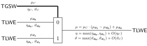
TheCMux gate has three input slots and one output slot: one control input slot represented by aTGSWsample on the integer message space (here restricted to{0,1}), twodata input slots each carrying aTLWEsample on the continuous message space TN[X], and one data output slot, also of type TLWE. The con-trolledMUXgateCMux(C,d1,d0) homomorphically outputs either the message of
d1 or d0 depending on the Boolean value in C, without decrypting any of the
three cipertexts. In practice, it returnsC (d1−d0) +d0.
In leveled circuits, the rule to build valid circuits usingCMuxgates (Figure 1) is that all control wires (TGSW) are freshly generated by the user, and the data input ports of our gates can be either freshly generated or connected to a data output or to another gate. In Section 6.2, we propose an efficient way to transform aTLWEsample in aTGSWsample, in order to make the circuits en-tirely composable (and so relax the condition requiring freshly generated control wires).
Lemma 3.16 (CMux gate). Let d0,d1 ∈ TLWEs(TN[X]) and C ∈
TGSWs({0,1}). Then msg(CMux(C,d1,d0)) = msg(C)?msg(d1):msg(d0).
Fur-thermore
– kErr(CMux(C,d1,d0))k∞≤max(kErr(d0)k∞,kErr(d1)k∞) +η(C),
– Var(Err(CMux(C,d1,d0))) ≤max(Var(Err(d0)),Var(Err(d1))) +ϑ(C), in the
conditions of Assumption 3.11,
TGSW
µC ηC,ϑC
TLWE
µd0 ηd0,ϑd0
TLWE
µd1 ηd1,ϑd1
0
1
TLWE
µ=µC·(µd1−µd0) +µd0 η= max(ηd0, ηd1) +O(ηC) ϑ= max(ϑd0, ϑd1) +O(ϑC)
Fig. 1. CMux gate -The CMux gate takes in input a TGSW sampleC with message
µC, aTLWEsampled0 with message µd0 and aTLWEsampled1with message µd1. It outputs aTLWEsample with messageµ=µC·(µd1−µd0) +µd0. Theη’s andϑ’s represent respectively the noise in the worst and average case, for both the inputs and the output.
Proof. The formulas for the noise in the worst and average cases are a conse-quence of Theorem 3.13 and Corollary 3.14. However, we need to explain why there is a max instead of the sum we would obtain by blindly applying these results. Letd=d1−d0, recall that in the proof of Theorem 3.13, the expression
ofC dis DecH,β,(d)•ZC+µCdec+µCzd+ (0, µC·µd), whereC=ZC+µC·H andd=zd+ (0, µd),ZC and zd are respectivelyTGSWandTLWEsamples of 0, andkdeck∞≤. Thus,CMux(C,d1,d0) is the sum of four terms:
– DecH,β,(d)•ZC of norm≤(k+ 1)`N βηC; – µCdec of norm≤(kN + 1);
– zd0+µC(zd1−zd0), which is eitherzd1 orzd0, depending on the value ofµC; – (0, µd0+µC·(µd1−µd0)), which is the trivial sample of the output message
µC?µd1:µd0, and is not part of the noise.
Thus, summing the three terms concludes the proof. For the average case, the formula is proven in the same way by using the results of Corollary 3.14 and replacing all norm inequalities by variance inequalities. ut
Notations In the rest of the paper, the notation TLWEis used to denote the (canonical scalar) binary TLWE problem (i.e. the LWE problem described in Section 2). To distinguish it from the Ring mode, we introduce the notation
TRLWE. TheTGSWsamples are only used in ring mode, but we use the notation
TRGSW to keep uniformity with theTRLWEnotation.
Furthermore, we distinguish theTLWEkeys from theTRLWE keys by using the respective notationsKand K, instead of the genericsused until now. We also use the following convention in the rest of the paper: for all n = kN, a binary vector K∈ Bn can be interpreted as a TLWEkey, or alternatively as a
TRLWEkeyK∈BN[X]khaving the same sequence of coefficients. Namely,Kiis the polynomialPN−1
4
Building blocks for TFHE
TLWE and TRLWE samples are largely used in the rest of the paper, and the schemes we describe switch from a type to another constantly. To do that, three basic tools are used: the key switching, the sample extraction and the blind rotation. Each one of them is described in detail in next sections.
4.1 Key Switching revisited
We revisit the well-known key switching procedure, largely described in the literature. The principal interest of key switching, as the name suggests, is to switch between keys in different parameter sets.
We show that this procedure has a larger potential. It allows to switch be-tween the scalar and polynomial message spacesTandTN[X], and more gener-ally, it has the ability to homomorphically evaluate linear morphismsf from any Z-moduleTp to TN[X]. We define two key switching flavors, one for a publicly knownf, and one for a secret f encoded in the key switching key.
In the following, we denotePubKS(f,KS,c) andPrivKS(KS(f),c) the output of Algorithm 2 and Algorithm 3, taking in input the functional key switching keysKSandKS(f)respectively and aTLWEciphertextc.
As the inputs and the outputs are instantiated with different parameter sets and we want to keep the same name for the variablesn, N, α, `, Bg, . . ., we add an under bar to the output parameters to distinguish them from the input pa-rameters.
From now on, we use the letter γ to indicate the standard deviation of the key-switching key. The variablet represents the precision of the binary decom-position.
Algorithm 2TLWE-to-T(R)LWE Public Functional Key Switching
Input: pTLWEciphertextsc(z)= (a(z),b(z))∈TLWEK(µz) forz= 1, . . . , p, a public
R-Lipschitz morphismf:Tp→TN[X], andKSi,j∈T(R)LWEK(
Ki
2j).
Output: AT(R)LWEsamplec∈T(R)LWEK(f(µ1, . . . , µp))
1: fori∈[[1, n]]do
2: Letai=f(a (1) i , . . . ,a
(p) i )
3: let ˜aibe the closest multiple of 21t toai, thusk˜ai−aik∞<2 −(t+1)
4: Binary decompose each ˜ai=Ptj=1˜ai,j·2−jwhere ˜ai,j∈BN[X]
5: end for
6: return(0, f(b(1), . . . ,b(p)))−Pn i=1
Pt
j=1˜ai,j·KSi,j
Theorem 4.1. (Public Key Switching) Given p TLWE ciphertexts c(z) ∈ TLWEK(µz), a public R-Lipschitz morphism f : Tp → TN[X] of Z-modules, andKSi,j ∈T(R)LWEK,γ(
Ki
– kErr(c)k∞≤RkErr(c)k∞+ntNAKS+n2−(t+1) (worst case), – Var(Err(c))≤R2Var(Err(c)) +ntN ϑKS+n2−2(t+1) (average case),
where AKS andϑKS=γ2 are respectively the amplitude and the variance of the
error of KS.
Proof. Letcbe the output of Algorithm 2 and b=f(b(1), . . . ,b(p)) then
ϕK(c) =b−
n X i=1 t X j=1 ˜
ai,j·ϕK(KSi,j)
=b−
n X i=1 t X j=1 ˜ ai,j(Ki
2j −Err(KSi,j)) =b−
n
X
i=1
Ki˜ai−
n X i=1 t X j=1 ˜
ai,jErr(KSi,j)
=b−
n
X
i=1
Kiai−
n X i=1 t X j=1 ˜
ai,jErr(KSi,j) + n
X
i=1
Ki·(ai−ai)˜
=f(b(1), . . . ,b(p))−
n
X
i=1
f(a(1)i , . . . ,a(p)i )Ki
− n X i=1 t X j=1 ˜
ai,jErr(KSi,j) + n
X
i=1
Ki·(ai−ai)˜
=f (b(1), . . . ,b(p))−
n
X
i=1
Ki(a
(1) i , . . . ,a
(p) i ) ! − n X i=1 t X j=1 ˜
ai,jErr(KSi,j) + n
X
i=1
Ki·(ai−ai)˜
=f(ϕK(c(1))), . . . , ϕK(c(p)))− n X i=1 t X j=1 ˜
ai,jErr(KSi,j) + n
X
i=1
Ki·(ai−a˜i)
Applying the expectation on each side, we obtain msg(c) on the left, and f(µ1, . . . , µp) on the right, since all the error terms have expectation 0 and f is linear. For the worst-case bound, we obtain that:
kErr(c)k∞=ϕK(c)−msg(c)
∞
≤ f(Err(c
(1)), . . . ,Err(c(p)))
∞+ntNAKS+N n2
−(t+1)
≤RkErr(c)k∞+ntNAKS+N n2−(t+1)
sincef is R-Lipschitz. For the average-case, we have a similar proof:
Var(Err(c)) =Var(ϕK(c)−msg(c))
≤Var(f(Err(c(1)), . . . ,Err(c(p)))) +ntN ϑKS+N n2−2(t+1)
≤R2Var(Err(c)) +ntN ϑKS+N n2−2(t+1).
Remark 2. TheTLWE-to-T(R)LWEpublic key switching procedure we described, allows to switch between the scalar message spaceTand the polynomial message space TN[X]. The same procedure can be used to perform a TLWE-to-TLWE public key switching and switch between scalar message spaces. Here is why we put parentheses around the Rof T(R)LWE. In practice, the key switching key is composed by TLWE encryptions of the old secret key, and the noise growth formulas remain the same, with the factorN equal to 1. We use the TLWE
-to-TLWEpublic key switching in Section 5.3. Furthermore, observe that the public key-switching procedure can be used from TRLWE to TRLWE: in this case the functionf is just the identity function.
We have a similar result when the function is private. In this algorithm, we extend the input secret keyKby adding a (n+ 1)-th coefficient equal to−1, so that ϕK(c) =−K·c.
Algorithm 3TLWE-to-T(R)LWE Private Functional Key Switching Input: p TLWE ciphertexts c(z) ∈ TLWE
K(µz), a key switching key KS(f)z,i,j ∈ T(R)LWEK(f(0, . . . ,0,Ki
2j,0, . . . ,0)) wheref:T
p→
TN[X] is a secret R-Lipschitz
morphism and Ki
2j is at positionz(also,Kn+1=−1 by convention). Output: AT(R)LWEsamplec∈T(R)LWEK(f(µ1, . . . , µp)).
1: fori∈[[1, n+ 1]],z∈[[1, p]]do
2: Let ˜c(z)i be the closest multiple of 1 2t toc
(z)
i , thus|˜c (z) i −c
(z) i |<2
−(t+1)
3: Binary decompose each ˜c(z)i =
Pt j=1˜c
(z) i,j ·2
−j
where ˜c(z)i,j ∈ {0,1}
4: end for
5: return−Pp z=1
Pn+1 i=1
Pt j=1˜c
(z) i,j ·KS
(f) z,i,j
Theorem 4.2. (Private Key Switching) Given p TLWE ciphertexts c(z) ∈ TLWEK(µz), and KS(f)i,j ∈ T(R)LWEK,γ(f(0, . . . ,Ki
2j, . . . ,0)) where f : T
p →
TN[X] is a private R-Lipschitz morphism of Z-modules, Algorithm 3 outputs aT(R)LWEsample c∈T(R)LWEK(f(µ1, . . . , µp))such that:
– kErr(c)k∞≤RkErr(c)k∞+ (n+ 1)R2−(t+1)+pt(n+ 1)A
KS (worst-case),
– Var(Err(c)) ≤ R2Var(Err(c)) + (n+ 1)R22−2(t+1)+pt(n+ 1)ϑ
KS (average
case),
Proof. Letcbe the output of Algorithm 3 and b=f(b(1), . . . ,b(p)) then:
ϕK(c) =− p X z=1 n+1 X i=1 t X j=1 ˜
c(z)i,j ·ϕK(KS (f) z,i,j) =− p X z=1 n+1 X i=1 t X j=1 ˜ c(z)i,j
f(0, . . . ,Ki
2j, . . . ,0) +Err(KS (f) i,j) =− p X z=1 n+1 X i=1 t X j=1 ˜
c(z)i,jf(0, . . . ,Ki
2j, . . . ,0)− p X z=1 n+1 X i=1 t X j=1 ˜
c(z)i,jErr(KS(f)z,i,j)
We setKS=P
p z=1
Pn+1
i=1
Pt
j=1c˜ (z) i,jErr(KS
(f)
z,i,j). Then:
=− n+1 X i=1 p X z=1
f(0, . . . , t
X
j=1 ˜ c(z)i,jKi
2j, . . . ,0)−KS
=− n+1 X i=1 p X z=1
f(0, . . . ,Ki·c˜ (z) i , . . . ,0)
− n+1 X i=1 p X z=1
f(0, . . . ,Ki·(˜c (z) i −c
(z)
i ), . . . ,0)−KS
=−
n+1
X
i=1
Kif(c(1)i , . . . ,c(z)i , . . . ,c(p)i )−
n+1
X
i=1
Kif(˜c(1)i −c(1)i , . . . ,˜c(p)i −c(p)i )−KS
=f(−
n+1
X
i=1
Kic
(1) i , . . . ,−
n+1
X
i=1
Kic
(p) i )−
n+1
X
i=1
Kif(˜c(1)i −c(1)i , . . . ,˜c(p)i −c(p)i )−KS
=f(ϕK(c(1)), . . . , ϕK(c(p)))−
n+1
X
i=1
Kif(˜c(1)i −c(1)i , . . . ,˜c(p)i −c(p)i )−KS
=f(µ1+Err(c(1)), . . . , µp+Err(c(p)))
−
n+1
X
i=1
Kif(˜c(1)i −c(1)i , . . . ,˜c(p)i −c(p)i )−KS
By linearity off and since the expectation of the error terms are 0, the message of the right side is equal tof(µ1, . . . , µp). For the worst-case bound on the noise, asf is R-Lipschitz, we obtain:
kErr(c)k∞=ϕK(c)−msg(c) ∞
≤RkErr(c)k∞+ (n+ 1)R2−(t+1)+pt(n+ 1)AKS
4.2 Sample Extraction.
ATRLWE message is a polynomial withN coefficients, which can be viewed as N slots over T. It is easy to homomorphically extract a coefficient as a scalar
TLWE sample with the same key. We recall that a binary TLWE key K ∈ Bn can be interpreted as a TRLWEkey K ∈BN[X]k having the same sequence of coefficients, and vice-versa.
Given a TRLWE sample c = (a, b) ∈ TRLWEK(µ) and a position p ∈ [0, N−1], we callSampleExtractp(c) theTLWEsample (a,b) whereb=bp and
aN(i−1)+j+1is the (p−j)-th coefficient ofai (using theN-antiperiodic indexes). This extracted sample encodes the p-th coefficient µp with at most the same noise variance or amplitude asc. In the rest of the paper, we will simply write
SampleExtract(c) whenp= 0.
In Section 5, we show how theKeySwitchingand theSampleExtractprocedures are used to efficiently pack data, unpack and move data across the slots, and how it differs from usual packing techniques.
4.3 Blind Rotate
The BlindRotate algorithm multiplies the polynomial encrypted in the input
TRLWEciphertext by an encrypted power ofX. The effect produced is a rotation of the coefficients. The algorithm consists in two parts. The first one (line 3) is the rotation by a known power of X The second one (loop at line 4) is the rotation by a secret power of X, which is performed by using the CMux gate, described in Section 3.4.
Algorithm 4BlindRotate
Input: ATRLWEsamplecofv∈TN[X] with keyK.
1: p+ 1 int. coefficientsa1, . . . , ap, b∈Z/(2NZ)
2: pTRGSWsamplesC1, . . . , Cpofs1, . . . , sp∈Bwith keyK
Output: ATRLWEsample ofX−ρ·vwhereρ=b−Pp
i=1si.ai mod 2N with keyK
3: ACC←X−b•c
4: fori= 1top
5: ACC←CMux(Ci, Xai·ACC,ACC)
6: returnACC
Theorem 4.3. Let H ∈ M(k+1)`,k+1(TN[X]) the gadget matrix and DecH,β, its efficient approximate gadget decomposition algorithm with qualityβ and pre-cision defining TRLWE and TRGSW parameters. Let α ∈ R≥0 be a noise parameter, K ∈ Bn be a TLWE secret key and K ∈
BN[X]k be its TRLWE interpretation. Given one sample c ∈ TRLWEK(v) with v ∈ TN[X], p+ 1 integers a1, . . . , ap and b ∈ Z/2NZ, and p TRGSW ciphertexts C1, . . . , Cp, where each Ci ∈ TRGSWK,α(si) for si ∈ B. Algorithm 4 outputs a sample
– kErr(ACC)k∞≤ kErr(c)k∞+p(k+ 1)`N βAC+p(1 +kN)(worst case), – Var(Err(ACC))≤Var(Err(c)) +p(k+ 1)`N β2ϑC+p(1 +kN)2 (average case), whereϑC=α2 andAC are the variance and amplitudes of Err(Ci).
Proof. Theorem 4.3 follows from the fact that algorithm 4 callsptimes theCMux
evaluation. ut
We define BlindRotate(c,(a1, . . . , ap, b),(C1, . . . , Cp)), the procedure de-scribed in Algorithm 4 that outputs theTRLWEsampleACCas in Theorem 4.3.
5
Leveled Homomorphic Encryption
The main goal of Homomorphic Encryption is to perform computations on en-crypted data. In previous sections we described all the different tools to ma-nipulate the ciphertexts. In this section we show how to use them to construct homomorphic circuits. In particular, we describe the evaluation of a random function via its look-up table and we propose two packing techniques that can be used to accelerate the evaluation.
Various packing techniques have already been proposed for homomorphic encryption: the Lagrange embedding in Helib [37, 36], the diagonal matrices en-coding in [46] or the CRT enen-coding in [49, 50, 10]. The message space is often a finite ring (e.g.Z/pZ), and the packing function is in general chosen as a ring isomorphism that preserves the structure of (Z/pZ)N. This way, elementary ad-ditions or products can be performed simultaneously on N independent slots, and thus, packing is in general associated to the concept of batching a single operation on multiple datasets. These techniques can have some limitations, es-pecially if in the whole program, each function is only run on a single dataset, and most of the slots are unused. This is particularly true in the context of
GSW evaluations, where functions are split into many branching algorithms or automata, that are each executed only once.
In the rest of the paper, packing refers to the canonical coefficients em-bedding function, that mapsN TLWEmessages µ0, . . . , µN−1∈Tinto a single
TRLWEmessageµ(X) =PN−1
i=0 µiX
i. This function is a
Z-module isomorphism. Messages can be homomorphically unpacked from any slot using the (noiseless)
SampleExtractprocedure, described in Section 4.2. Reciprocally, we can repack, move data across the slots, or clear some slots by using our public functional key switching from Algorithm 2 to evaluate respectively the canonical coeffi-cient embedding function (i.e. the identity), a permutation, or a projection. Since these functions are 1-Lipschitz, by Theorem 4.1, these keyswitch opera-tions only induce a linear noise overhead. It is arguably more straightforward than the permutation network technique used in Helib. But as in [10, 18, 26], our technique relies on a circular security assumption, even in the leveled mode since our keyswitching key encrypts its own key bits12.
12
We now analyze how packing can speed-up TRGSW leveled computations, first for look-up tables or random functions, and then for most arithmetic func-tions.
5.1 Arbitrary functions and Look-Up Tables
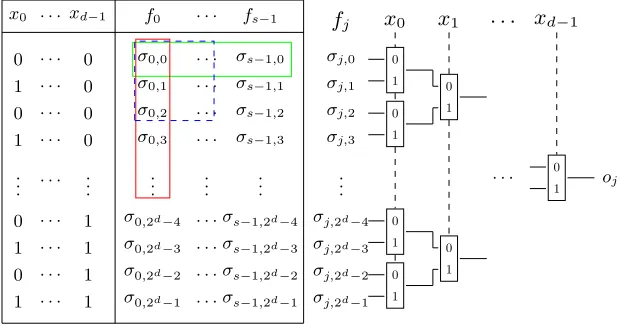
The first class of functions we analyze are arbitrary functionsf :Bd→Ts. Such functions can be expressed via a Look-Up Table (LUT), containing the list of 2d input values (each one composed by d bits) and corresponding LUT values for the s sub-functions (1 element in T per sub-function fj). We denote the LUT values with σj,h ∈T, where j ∈[[0, s−1]] is the sub-function index, and h∈[[0,2d−1]] is the input index.
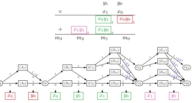
In order to computef(x) = (f0(x), f1(x), . . . , fs−1(x)), wherex=P d−1 i=0 xi2i is a d-bit integer, the classical evaluation of such function, as proposed in [15, 22], consists in evaluating thessub-functionsf0, f1, . . . , fs−1separately. Each of them consists in a binary decision tree composed by 2d−1CMuxgates. The total complexity of the classical evaluation requires therefore to execute abouts·2d CMuxgates. Let’s calloj=fj(x)∈Tthej-th output off(x), forj= 0, . . . , s−1. Figure 2 summarizes the idea of the computation ofoj.
In this section we present two techniques, that we call horizontal and vertical packing, that can be used to improve the evaluation of a LUT. The packing technique is the same in both cases: the idea is to packN TLWEmessages inside the polynomial coefficients of a singleTRLWEciphertext. The names horizontal and vertical refer to the two different ways to use such packing. Intuitively, they describe in which sense the data of the LUT are packed and manipulated in order to evaluate the functionf.
Horizontal packing corresponds exactly to batching. In fact, it exploits the fact that thessub-functions evaluate the sameCMuxtree, with the same inputs but with the different LUT values corresponding to thestruth tables. For each of the 2d possible input values, we pack the LUT values of thes sub-functions in the first s slots (i.e. in the first s coefficients of the polynomial) of a single
TRLWE ciphertext (the remainingN−sare unused). By using a single 2d size CMux tree to select the right ciphertext, we obtain thesslots all at once, which is overallstimes faster than the classical evaluation.
On the other hand, our vertical packing is very different from the batching techniques. The basic idea is to pack several LUT values of a single sub-function in the same ciphertext, and to use bothCMuxand blind rotations to extract the desired value. Unlike batching, this can also speed up functions that have only a single bit of output.
In the following we detail these two techniques. They can be used both sep-arately or combined, depending on the application.
x0 . . . xd−1 f0 . . . fs−1
0 . . . 0 σ0,0 . . . σs−1,0 σj,0
1 . . . 0 σ0,1 . . . σs−1,1 σj,1
0 . . . 0 σ0,2 . . . σs−1,2 σj,2
1 . . . 0 σ0,3 . . . σs−1,3 σj,3
. .
. . . . ... ... ... ... ...
0 . . . 1 σ0,2d−4 . . . σs−1,2d−4 σj,2d−4
1 . . . 1 σ0,2d−3 . . . σs−1,2d−3 σj,2d−3
0 . . . 1 σ0,2d−2 . . . σs−1,2d−2 σj,2d−2
1 . . . 1 σ0,2d−1 . . . σs−1,2d−1 σj,2d−1
0
1
0
1
0
1
0
1 0
1
0
1
. . . 0
1 oj
f
jx
0x
1. . . x
d−1Fig. 2. LUT with CMuxtree -Intuitively, the horizontal rectangle encircles the bits packed in the horizontal packing, while the vertical rectangle encircles the bits packed in the vertical packing. The dashed square represents the packing in the case where the two techniques are mixed. The right part of the figure represents the evaluation of the sub-functionfj onx=Pi=0d−1xi2i via aCMuxbinary decision tree.
noise propagation in the binary decisionCMuxtree has already been given in [31] and [22].
Horizontal Packing (or Batching) The idea of the horizontal packing is to evaluate all the outputs of the functionf together, instead of evaluating all the fj separately. This is possible by using TRLWE samples, as the message space isTN[X]. In fact, we could encrypt up to N LUT valuesσj,h (for a fixed h ∈ [[0,2d−1]]) per TRLWE sample and evaluate the binary decision tree as described before. The number of CMux gates to evaluate is ds
Ne(2
d−1). This technique is optimal if the sizesof the output is a multiple ofN. Unfortunately, s is in general ≤N and the number of gates to evaluate remains 2d−1. The evaluation of the function f is then only s times faster than the non-packed approach. As not all the slots are used, this technique it is not optimal if s is small. The elementary Lemma 5.1 specifies the noise propagation and it follows immediately from Lemma 3.16 and from the construction of the binary decision CMux tree, which has depthd.
Lemma 5.1 (Horizontal Packing - Batching).Letd0, . . . ,d2d−1beTRLWE
samples13 such thatd
h∈TRLWEK(P s
j=0σj,hXj) forh∈[[0,2d−1]]. Here the σj,h are the LUT values relative to an arbitrary function f : Bd → Ts. Let C0, . . . , Cd−1 beTRGSWsamples, such thatCi∈TRGSWK(xi)withxi∈B(for
13
i∈[[0, d−1]]), andx=Pd−1
i=0xi2i. Let dbe theTRLWE sample output by thef evaluation of the binary decision CMux tree for the LUT (described in figure 2). Then, using the same notations as in Lemma 3.16 and settingmsg(d) =f(x):
– kErr(d)k∞≤ ATRLWE+d·((k+ 1)`N βATRGSW+ (kN+ 1))(worst case),
– Var(Err(d))≤ϑTRLWE+d·((k+ 1)`N β2ϑTRGSW+ (kN+ 1)2)(average case),
where ATRLWE andATRGSW are upper bounds of the infinite norm of the errors
of the TRLWE samples and the TRGSW samples respectively and ϑTRLWE and
ϑTRGSW are upper bounds of their variances.
Vertical Packing In order to improve the evaluation of the LUT, we propose a second optimization calledVertical Packing. As for the horizontal packing we use the TRLWE encryption to encode N values at the same time. But now, instead of packing the LUT values σj,h with respect to a fixed h∈ [[0,2d−1]] i.e. “horizontally”, we pack N values σj,h “vertically”, with respect to a fixed j∈[[0, s−1]]. Then, instead of just evaluating a fullCMuxtree, we use a different approach.
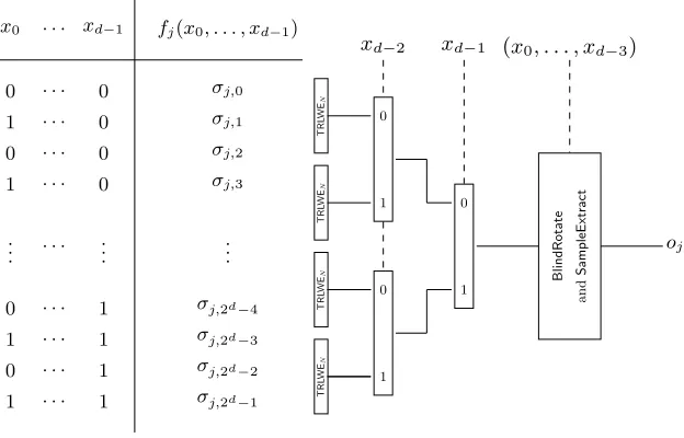
If the LUT values are packed in “boxes”, our technique first uses a packed CMuxtree to select the right box, and then, a blind rotation (Algorithm 4) to find the right element inside the selected box. Figure 3 gives a schematic overview of the entire procedure.
Now, suppose that one wants to evaluate the functionf, or just one of its sub-functionsfj, on a fixed inputx=Pd−1
i=0 xi2
i. We assume the LUT associated to fj is known as in figure 2. The output offj(x) is just the LUT valueσj,x at positionx.
Let δ = log2(N). We analyze the general case where 2d is a multiple of N = 2δ. The LUT offj, which is a column of 2d values, is now packed as 2d/N
TRLWEciphertextsd0, . . . ,d2d−δ−1, where eachdk encodesN consecutive LUT valuesσj,kN, . . . , σj,(k+1)N−1. To retrievefj(x), we first need to select the block
that contains σj,x. This block has index p= bx/Nc, whose bits are the d−δ most significant bits ofx. Since theTRGSWencryptions of these bits are among our inputs, one can use a CMux tree to select this block dp. Then, σj,x is the ρ-th coefficient of the message of dp where ρ = x modN = P
δ−1
i=0xi2i. The bits ofρare theδleast significant bits ofx, which are also available asTRGSW
ciphertexts in our inputs. We can therefore use a blind rotation (Algorithm 4) to homomorphically multiply dp by X−ρ, which brings the coefficient σj,x in position 0, and finally, we extract it with a SampleExtract. Algorithm 5 details the evaluation offj(x).
The entire cost of the evaluation offj(x) with Algorithm 5 consists in 2Nd−
1 CMux gates and a single blind rotation, which corresponds to δ CMux gates. Overall, we get a speed-up by a factor N on the evaluation of each partial function, so a factorN in total.
Lemma 5.2 (Vertical Packing LUT of fj). Let fj : Bd → T be a sub-function of the arbitrary function f : Bd → Ts, with LUT val-ues σj,0, . . . , σj,2d−1. Let d0, . . . ,d2d
N−1
x0 . . . xd−1 fj(x0, . . . , xd−1)
0 . . . 0 σj,0
1 . . . 0 σj,1
0 . . . 0 σj,2
1 . . . 0 σj,3
. .
. . . . ... ...
0 . . . 1 σj,2d−4
1 . . . 1 σj,2d−3
0 . . . 1 σj,2d−2
1 . . . 1 σj,2d−1
TRL
WE
N
TRL
WE
N
TRL
WE
N
TRL
WE
N
0
1
0
1
0
1 BlindRotate
and
SampleExtract
oj
xd−2 xd−1 (x0, . . . , xd−3)
Fig. 3. Vertical packing for the evaluation of the fj LUT - As described in
Algorithm 5, the image represents the idea of evaluation of the sub-function fj on x = Pd−1
i=0xi2 i
via vertical packing technique. After “vertically” packing the LUT valuesσj,h(forh∈[[0,2d−1]]) in groups of sizeN, insideTRLWEsamples, aCMuxtree,
a blind rotation and a sample extract are evaluated. TheCMuxtree is initially used to select theTRLWEsample containing the output value. Then the output value is moved in the place of the constant coefficient of theTRLWEmessage by using the blind rotation (Algorithm 4) and extracted by using the sample extraction (Section 4.2). The bits of
xare given asTRGSWsamples and the final resultoj=fj(x) is extracted as aTLWE
sample. In our example, we fixed 2d= 4N.
TRLWEK(P N−1
i=0 σj,pN+iXi) forp∈[[0,2
d
N −1]]
14. LetC
0, . . . , Cd−1 beTRGSW samples, such thatCi∈TRGSWK(xi), withxi∈Band i∈[[0, d−1]].
Then algorithm 5 outputs a TLWEsample csuch that msg(c) =fj(x) =oj where x = Pd−1
i=0 xi2i and using the same notations as in Lemma 3.16 and Theorem 4.3, we have:
– kErr(d)k∞≤ ATRLWE+d·((k+ 1)`N βATRGSW+ (1 +kN))(worst case),
– Var(Err(d))≤ϑTRLWE+d·((k+ 1)`N β2ϑTRGSW+ (1 +kN)2)(average case),
where ATRLWE andATRGSW are upper bounds of the infinite norm of the errors
in the TRLWE samples ant the TRGSW samples respectively, while ϑTRLWE and
ϑTRGSW are upper bounds of the variances.
14
If the sub-functionfj and its LUT are public, the LUT valuesσj,0, . . . , σj,2d−1 can
be given in clear. This means that theTRLWEsamplesdp, forp∈[[0,2
d
N −1]] are
given as trivialTRLWEsamplesdp←(0,PN
−1
Algorithm 5Vertical Packing LUT offj :Bd→T(calling algorithm 4) Input: A list of 2Nd TRLWEsamplesdp∈TRLWEK(Pi=0N−1σj,pN+iXi) forp∈[[0,2
d
N−
1]], a list ofdTRGSWsamplesCi∈TRGSWK(xi), withxi∈Bandi∈[[0, d−1]],
Output: ATLWEsamplec∈TLWEK(oj=fj(x)), withx=Pdi=0−1xi2i
1: Evaluate the binary decision CMux tree of depth d−δ, with TRLWE inputs
d0, . . . ,d2d N−1
andTRGSWinputsCδ, . . . , Cd−1, and output aTRLWEsampled
2: d←BlindRotate(d,(20, . . . ,2δ−1,0),(C0, . . . , Cδ−1))
3: Return c=SampleExtract(d)
Proof. The proof follows immediately from the results of lemma 3.16 and theo-rem 4.3, and from the construction of the binary decisionCMuxtree. In particular, the firstCMuxtree has depth (d−δ) and the blind rotation evaluatesδCMuxgates, which brings a total factordin the depth. As theCMux depth is the same as in horizontal packing, the noise propagation matches too. ut
Remark 4. As previously mentioned, the horizontal and vertical packing tech-niques can be mixed together to improve the evaluation off. This combination is optimal in the case wheresanddare both small or if 2d·s > N. In particular, if we pack x = s coefficients horizontally and y = N/x coefficients vertically, we needd2d/ye −1 CMuxgates plus one vertical packing LUT evaluation in or-der to evaluate f, which is equivalent to log2(y) CMux evaluations. The result is composed of the first xTLWEsamples extracted. A practical example of the combination of the two techniques is given in Section 5.3.
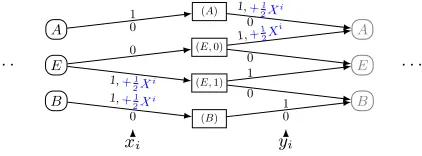
5.2 Deterministic automata
It is folklore that every deterministic program which reads its input bit-by-bit in a pre-determined order, uses fewer than B bits of memory, and produces a Boolean answer, is equivalent to a deterministic automata of at most 2B states (independently of the time complexity). This is in particular the case for every Boolean function of pvariables, that can be trivially executed with p−1 bits of internal memory by reading and storing its input bit-by-bit before returning the final answer. It is of particular interest for most arithmetic functions, like addition, multiplication, or CRT operations, whose naive evaluation only requires O(log(p)) bits of internal memory.
But when message space is not binary, and several bits are packed together as we show in previous sections, a more powerful tool is needed to manage the evaluations in an efficient way.
![Table 1. TFHE elementary operations - In this table, allcTTheTthe µi’s denote plaintexts inN[X] and ci the corresponding TRLWE ciphertext](https://thumb-us.123doks.com/thumbv2/123dok_us/7982153.1324071/49.612.133.504.115.256/table-elementary-operations-allctthetthe-denote-plaintexts-corresponding-ciphertext.webp)
![Table 4. New Parameters and security of the Gate bootstrapping - This tableshows the parameters for the keyswitching key and the bootstrapping key based on therecent cost models recommended in the homomorphic encryption security standard[1]](https://thumb-us.123doks.com/thumbv2/123dok_us/7982153.1324071/55.612.146.463.116.159/parameters-bootstrapping-tableshows-keyswitching-bootstrapping-recommended-homomorphic-encryption.webp)
