SinoTERM365, Bottom-up Representation of China at the Prefectural Level

SinoTERM365, Bottom-up Representation of China

at the Prefectural Level

CoPS Working Paper No. G-285, October 2018

The Centre of Policy Studies (CoPS), incorporating the IMPACT project, is a research centre at Victoria University devoted to quantitative analysis of issues relevant to economic policy. Address: Centre of Policy Studies, Victoria University, PO Box 14428, Melbourne, Victoria, 8001 home page: www.vu.edu.au/CoPS/ email: [email protected] Telephone +61 3 9919 1877

Glyn Wittwer

And

Mark Horridge

Centre of Policy Studies, Victoria University

1

SinoTERM365, bottom-up

representation of China at the

prefectural level

The TERM methodology requires relatively modest data requirements to create a multi-regional, sub-national CGE database. SinoTERM365 is an extreme form of stretching available data, with the master database representing 162 sectors in 365 prefectural regions of the Chinese economy. A collaborative effort is envisaged among users to enable ongoing improvements to the database. The TERM approach facilitates rapid amendments to the database when improved data are available. The alternative, to wait until better data emerge before building a model, may result in less detail and a less versatile framework for analysis. In our example, we consider a downturn in use of coal and coal-generated electricity in China.

JEL codes: C68, D58, R13, R15

2

Table of contents

1. Introduction 3

2. The TERM approach 6

2.1 Comparison with the GTAP model 9 2.2 The TERM data strategy 9 2.3 Preparation of national database 10 2.4 Estimates of the regional distribution of output and final demands 11 2.5 The TRADE matrix 15 2.6 Aggregation 16

3. The equations of TERM 17

3.2 Commodity sourcing at the sub-national level 20 3.3 Household demands 25 3.4 Investment demands 28 3.5 Other final demands 30

3.6 Margins 31

3.7 Market clearing equations and macro equations 33

4. Previous multi-regional models using the TERM approach 35 5. Simulation: Reducing China’s Use of Coal 38

5.1 Background to scenario 38 5.2 The scenario 39 5.3 Database issues 40 5.4 Should a large country face infinitely elastic import supplies in a national model? 41

6. Potential Model Developments 42

References 45

Tables

1. Summary of prefecture-level data quality 14

2. Definitions of variables, values and parameters in intermediate and final usage 19

3. Definitions of variables, values and parameters in trade 20

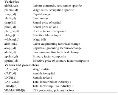
4. Definitions of variables, values and parameters in primary factor demands 21

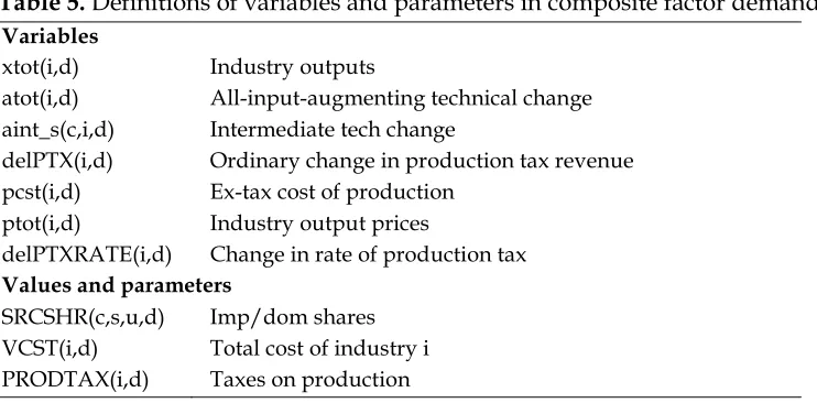
5. Definitions of variables and parameters in composite factor demands 23

6. Definitions of variables and parameters in industry supplies 25

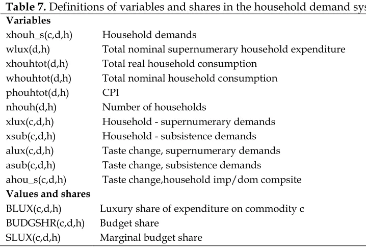
7. Definitions of variables and shares in the household demand system 27

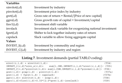
8: Definitions of variables and shares in investment demands 29

9: Definitions of variables and parameters in other final demands 31

10. Definitions of variables, shares and parameters in margins 33

11. Definitions of variables, values & mappings in market clearing & macro equations 35

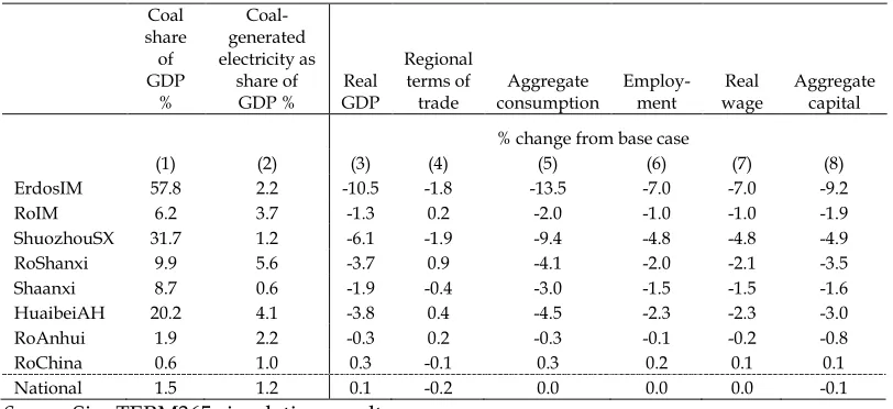
12. Long-run effects of 20% decrease in coal use and switch to hydropower 39

Figures

Figure 1. Aggregating from master database to policy simulation regions 17

3 1. Introduction

China’s economy provides a clear example of why sub-national detail is important in a CGE model. Not only are the populations of some provinces in excess of most countries in the world. The composition of the population is changing rapidly. The rural population is shrinking but remains large enough to be important on a global scale. Between 1980 and 2018, China’s population grew from 977 million to 1394 million, or 43 percent. This unremarkable statistic, given that global population grew by more than 70 percent in the same period, does not reveal the massive migration of workers from rural areas to cities. This has resulted in growth in some cities within a generation or two that is difficult to comprehend. In 1980, Shenzhen was a settlement of 58,000 surrounded by marshes, located over the border from Hong Kong. Over the next 20 years, Shenzhen transformed into a city of 7 million people. It has continued growing, reaching 11 million by 2018. Shenzhen’s neighboring city along the Pearl River delta, Dongguan, grew from 137,000 in 1980 to 7 million in 2018. In the corresponding period, the better known Pearl River delta city of Guangzhou grew from 1.9 million to 14.2 million. These are the biggest three cities/prefectures in Guangdong, a province with a population of a large nation and a GDP which now exceeds that of the Netherlands (International Monetary Fund, World Economic Outlook Database, April 2016 edition). In total, the province contains 21 prefectures, each with a population exceeding 1.5 million. In addition to the abovementioned cities, there are five others within the province with a population exceeding 5 million. Overall, Guangdong has a land area of around 177 thousand square kilometers, equivalent to the combined U.S. states of New York, New Jersey, Massachusetts and Connecticut but with almost 3 times the combined population of these four densely populated states.

4

transformed. Guiyang is being reinvented as a high-tech hub as the costs of living and doing business in eastern seaboard cities soar (Roxburgh 2017).

Some effects of urban change follow from the population growth. Compounding population pressures, rising incomes have resulted in rising per capita household spending. We can perceive China’s economic growth as both a miracle that has lifted hundreds of millions of people out of poverty and as an extreme strain on natural resources and infrastructure. In three decades from 1980, private car ownership increased 35-fold in per capita terms (Huang 2011). Frenzied road construction may not alleviate congestion in the face of rapid growth in private car use. Rising consumptions is also changing dietary habits: China now accounts for one quarter of global meat consumption (Myers 2016). An increase in demand for land and water follows from an increase in demand for meat. Yet the burgeoning cities are encroaching on farmland, so that high-rise buildings and other urban developments are displacing farm activity.

From the perspective of the rest of the world, China’s economic growth has buoyed global markets for mineral and agricultural products. Chinese investors have pursued land acquisitions in foreign nations as one way of coping with worsening land and water scarcity at home in the face of rising demand for food. China has changed the global economic structure, accelerating the shrinkage of manufacturing in developed nations at the same time as fueling a tourism boom as an increasing number of cashed-up Chinese citizens explore the world. The

GTAP model (Hertel 1997; Corong et al., 2017) is an invaluable tool for analyzing

the impacts that China is having on the rest of world. Our interest in the present study is to outline a model for analyzing sub-national impacts within China.

1.1 Analyzing regional economic issues in China

5

inland cities and the eastern seaboard, thereby contributing to improved

competitiveness in such cities.

Worsening water pollution is part of the broader issue of water

allocation. Lifestyle changes arising from growing incomes have resulted in

rapidly growing urban water demand. In common with the most of the rest

of the world, China has been reluctant to introduce market mechanisms to

assist in water allocation. In the medium term, increased demand for water

has accelerated groundwater extractions. Much of China’s response has

been through grand engineering schemes, notably the

South-to-North-Water-Diversion Project, which has brought water to water-scarce cities

including Beijing. There have been losers from the water diversion project,

notably the 330,000 people relocated from the surrounds of Danjiangkou

Reservoir in Shiyan prefecture, Hubei, in expansion of the reservoir arising

from the project. Local officials have described Danjiangkou city as the

“saddest city in China” accorded to China Daily (Wu Yan, 2014). In addition

to the relocation of inhabitants, many local industries important in regional

economic were closed down so as to reduce pollution of the water supply

arising from mining and manufacturing activities (Probe International,

2016)

Within provinces, some prefectures have boomed as others have lagged.

Shenzhen, Zhuhai and Shantou within Guangdong were designated as

“Special Economic Zones” in 1979 to attract foreign investment (Fan, 1995).

This resulted in these regions of China being the first to experience

accelerated growth: Shenzhen’s population has grown 190-fold since 1980,

compared with a 40-fold increase in Zhuhai and 10-fold increase in

Shantou. Growth in prefectures outside the Pearl River delta in Guangdong

was relatively slow in the earlier years of economic reform. More recently,

investments in transport infrastructure such as the Jieyang airport (So,

2008) have contributed to tourism growth in lagging regions of Guangdong.

6

has a corresponding share exceeding 20 percent. Agricultural output

grew

by around 5% per annum from the 1980s to 2007 (Wang

et al

., 2013), slower

than the rest of the economy: World Bank data indicate average annual real

GDP growth of 10% per annum between 1980 and 2007. This indicates that

provinces and prefectures in which agriculture had accounted for a large

share of total income are likely to grow relatively slowly. Agriculture has

to cope with worsening water and land scarcity, given the growing

demands of urban areas. Moreover, agriculture in some regions has

suffered from climate change. So while many cities boom, prefectures in

which agriculture remains important are vulnerable to stagnation or

decline, unless various adaptations are undertaken so that productivity

gains offset worsening input scarcity.

This paper presents details of SinoTERM365, a multi-regional model in

the TERM suite of sub-national models (Horridge

et al.

, 2005). The master

database of the model contains 162 sectors and 365 bottom-up

prefecture-based regions. The model has more sectors than the input-output table

published by China’s National Bureau of Statistics, with agriculture split

into different types of crops and livestock. In addition, the electricity sector

has been split into different types of generation, with a separate sector for

transmission and distribution.

Section 2 of the paper outlines the TERM approach to sub-national,

multi-regional CGE modeling. The theory of TERM is detailed in Section 3.

A summary of previous TERM-based models and studies follows in Section

4. Section 5 details the regional impacts of a downturn in coal use in China.

Section 6 concludes the paper with a discussion of potential applications of

SinoTERM365, including the inclusion of biophysical accounts at a

sub-national level.

2. The TERM approach

The TERM (The Enormous Regional Model) methodology circumvents two limitations that in the past have hindered sub-national multi-regional model development. The first is that as the number of sectors and regions increase, simulations may be slow. The second is that regional data may be scarce.

7

GTAP, the intermediate and final use matrices (a single matrix in the TERM format) include the regional user but not the regional origin. The trade matrices include the regional origin and regional destination but not the user. The small cost that comes with the common sourcing assumption is that the use matrices added up over users must equal the trade matrices summed across regional origins. The separation of full data dimensions into two matrices is an important distinction between TERM and Australia’s VURM (Adams et al. 2011), and

between GTAP (Hertel ,1997; Corong et al., 2017) and its predecessor SALTER

(Jomini, et al. 1994).

To illustrate the saving of using two matrices instead, consider a model in which there are 20 commodities, 20 industries, 4 final users and 20 sub-national regions plus imports. We assign a domestic and imported subscript to each origin so as to identify international port activity within the model. A use matrix identifying commodities (20), origins (20 x 2, i.e., domestic/imported), destinations (20), intermediate (20) plus final users (4) would contain 384,000 cells (=20x20x2x20x24). If we partition the data into a USE matrix excluding regional origins (20 commodities, 2 domestic\imported origins, 20 destinations and 24 users), with 19,200 cells and a TRADE matrix excluding users (20 commodities, 20 x 2 origins, 20 destinations) with 16,000 cells, the two matrices sum to 9.2% the size of a matrix that includes all relevant dimensions. The market clearing identity that enforces the two matrices to be equal will contain 800 cells (=20 commodities x 2 sources x 20 destinations) and therefore comes with only a small additional computational cost. Horridge (2011) provides more explanation of the structure of TERM and its sourcing mechanisms. Section 3 elaborates the equations including additional market-clearing equations required to implement the common sourcing assumption in TERM (see equations (53) to (55)).

In practice, a second strategy, that of aggregating sectors and regions of little or no interest in a scenario while maintaining detail in sectors and regions of interest, aids in rapid computational times. GTAP users took advantage of the common sourcing assumption and aggregation prior to the development of TERM.

The strategy to deal with scarce sub-national regional data is to keep the data requirements modest while using a reproducible sequence of problems, into which we can alter inputs readily as improved data emerge. The ORANI model (Dixon

8

industry-level production functions or inter-regional trade matrices, as is the case

in “bottom-up” representation, such as in TERM.The minimal data requirements

for constructing a TERM database are little more than those for a “top-down” multi-regional version of ORANI. Indeed, the standard procedure for preparing a TERM assumes that a working “top-down” database has already been prepared and used for simulations.

In the past, practitioners have often cited two constraints to regional modelling: these concern (1) the limited availability of regional IO tables, and (2) an absence of inter-regional trade detail.

In the case of China, IO tables are available for 30 regions (that is, all provinces [+4 municipalities] excluding Tibet). However, with one or two exceptions, notably Henan, the tables lack sectoral detail. Typically, agriculture, mining and manufacturing are each represented by little more than a single sector. Are these tables useful for control totals? To be useful, regional tables should sum to activities represented in the national table. The authors’ checks on China’s provincial tables indicate that they often do not sum reasonably to totals in the national table. This is not surprising, given that regional statistical bureaus prepare regional tables, with apparent limited harmonization between bureaus. But even with improved harmonization, a problem would remain, in that available regional IO tables do not take advantage of a great deal of regional data present in other sources. The TERM methodology is to make use of all available relevant data in preparing a multi-regional CGE database, and to allow for the possibility that as better data emerge, modelers can utilize it quickly in revising a CGE database. Section 2.4 details the data sources used in preparation of a disaggregated multi-regional CGE database.

9

invaluable though they may be in analysis of transport logistics, do not supersede the gravity method (outlined in Section 2.5) of allocating inter-regional trades in a regional CGE model.

Before providing more details on the TERM approach, from its inception we intended to apply this framework to a variety of countries. That is, the standard version of TERM avoids mechanisms that might be specific to a particular country or application, by retaining relative simplicity. Rather the emphasis is on allowing a basic multi-regional model to produce simulation results as soon as possible. Very often, analysis of results reveals shortcomings of the model or data, or suggests priorities for improvement. To arrive quickly at this stage is key to the quality of the final model. Section 4 lists the countries for which versions of TERM exist at present.

2.1 Comparison with the GTAP model

GTAP (Hertel, 1997; Corong et al., 2017) has a fairly similar structure to TERM.

The “regions” of GTAP, however, are countries or groups of countries, whilst in TERM they are regions within a single country. In GTAP, regional trade deficits must sum to zero [the planet is a closed system] whilst in TERM a national trade deficit is possible. There are also differences in data structures: GTAP has a far more detailed representation of bilateral trade taxes than does TERM, reflecting the freer trade that is usually possible within a nation. TERM can accommodate commodity tax rates that vary between regions (North might tax wine more than South) but it does not allow for regional tax discrimination (such as a tax, in North, that applied only to wine from West). Inter-regional labor movements, a rarity in GTAP, are usual in TERM. Finally, TERM has a more detailed treatment of transport margins. While GTAP identifies how much each country contributes to

world shipping supply, the TERM data structure shows how much each region contributes to supply of transport between all separate pairs of source and destination regions. Domestic margins are now being included in GTAP (Corong, 2018).

2.2 The TERM data strategy

TERM offers a strategy in stark contrast that of practitioners who believe that both regional IO tables and some inter-regional trade are necessary to devise a multi-regional CGE database. We have estimated the SinoTERM365 database from very limited regional data, even scarcer than the data typically used by TERM practitioners. Here we outline the strategy, while Section 2.4 outlines data sources.

The process starts with a national IO table and certain regional data. The

10

regions of industry outputs and of final demand aggregates. This distribution is based on a set of regional shares, which may in turn be calculated from value data, or on physical units (eg, tons of wheat) or on numbers employed. This flexibility (regarding units) greatly increases the amount of data that may be used. Additional regional detail, such as disaggregated sectoral shares from census data (which improve the quality of sectoral share estimates) or international trade by port, can be added when available.

The process is automated, so that additional detail can easily be added at a later stage. The database is constructed at the highest possible level of detail: 162 sectors and 365 regions in the case of SinoTERM365. Aggregation (for computational and presentational tractability) takes place at the end of the process, not at the beginning. Perhaps surprisingly, the high level of disaggregation is often helpful in estimating missing data. When aggregated, the model database displays a richness of structure that belies the simple mechanical rules that were used to construct its disaggregated parent. For example, even though we normally assume that a given disaggregated sector has the same IO coefficients wherever it is located, aggregated sectors display regional differences in technology. Thus, sectoral detail partly compensates for missing regional data.

Our technique of combining a national IO table with limited regional data to produce a detailed inter-regional table bears many similarities to methods developed over several decades by regional IO modellers. Indeed, published regional IO tables may well be in part constructed rather than observed. Unfortunately, the method of construction may be poorly documented or unrepeatable. Aspiring regional model developers may download the TERM data programs customize them to suit particular needs. They will appeal to the modeler who would prefer to construct a multi-regional database using known assumptions, rather than rely on data constructed somehow by others.

Published regional IO tables may well form part of the inputs to the TERM data process. But they should certainly not constrain the degree of regional or sectoral detail that we aim for.

2.3 Preparation of national database

11

the GTAP creators from the beginning wisely chose not to follow. The official Chinese IO table includes a single crops sector, a single livestock sector and another sector covering services to agriculture. We know that climate, water availability and types of crop vary widely across China. Moreover, even with rapid structural change, around 25% of China’s workforce (equal to 5% of the global workforce) is still employed in agriculture. Given that land and water availability is a major policy issue, we split the single crop sector from the available IO table into 14 and the single livestock sector into three. The meat sector is split into two to separate pork from other meat types. Within small regions, we may not know the share of national agricultural activity. But available data may provide good estimates of a region’s share of the 14 crops we have chosen to represent. Similarly, herd numbers and other statistics are available for various types of livestock.

A key assumption in the TERM methodology is that an identical technology or input cost structure is imposed on a given industry in all regions. For this assumption not to be burdensome, we undertake sectoral disaggregation at the national level beyond agriculture when it is obvious that technologies vary between regions. For example, hydroelectric generation dominates Sichuan’s electricity generation, whereas coal-fired generation dominates Shanxi’s generation. In preparing SinoTERM365’s database, we split electricity generation in the national database into seven different types of generation. To assume that coal generated electricity in Shanxi has the same technology as in Sichuan is defensible, whereas assuming that a single electricity generating sector in Shanxi has the same technology as Sichuan is not.

2.4 Estimates of the regional distribution of output and final demands

The first version of SinoTERM (Horridge and Wittwer, 2008; Wittwer and Horridge, 2009) represented the 27 provinces and 4 municipalities of China separately. But the populations of a number of Chinese provinces are so large that this remains a relatively coarse level of regional representation. Guangdong, for example, with 102 million inhabitants has a larger population than all but 13 countries. Shandong’s population of 95 million is similar to Vietnam’s. Third ranked province Henan, with 92 million, comfortably exceeds the population of

Germany (82 million), the world’s 16th most populous nation (from

http://population.city).

12

at a national level in only 32 other countries)1 _{and a median population of 37.3 for}

the 31 province-based regions. The prefectural representation, while stretching available data, uses regions with populations closer in magnitude to those of sub-national regions in other TERM-based models.

The idea for a prefectural level SinoTERM arose from a short course held in Beijing in July 2017. A number of participants expressed a desire to build their own database. CoPS made the database generation programs publicly available over a

decade ago (see https://www.copsmodels.com/archivep.htm#tpmh0067). The

authors thought it preferable to devise a large master database with the objective of providing access to a community of users in China. In this respect, the approach has been inspired by that of the GTAP community. We anticipate that a better database will emerge from a collaboration between different users involved in research on the Chinese economy than if each group builds their own database. Another advantage of this approach is that provision of a basic model will free up research resources for scenarios and CGE analysis. In addition, a basic highly disaggregated database will reduce the effort required to add model extensions such as greenhouse gas, energy or water accounts to a model. This does not mean that developers will preserve all sectoral detail as they add satellites. Rather, it is more likely that the core database will have good coverage of key sectors for particular accounts. For example, a model with greenhouse gas accounts may require some detailed representation of electricity generation, various types of metal production, livestock production and cement production. The developer may choose to aggregate sectors in which greenhouse gas accounts are less important.

As discussed in Section 2.3, the TERM approach is first to disaggregate the national IO table/CGE database. The regional shares required for each sector for devising SinoTERM are production shares of national activities, investment shares (set equal to production shares), household consumption shares, export shares, government spending shares and import shares. We examine data sources for production shares first. The primary source for regional data is Chinadataonline.org (China Data Center, University of Michigan), accessed via the National Library of Australia. In particular, the site provides access to provincial statistical yearbooks.

One of the strengths of the statistical yearbooks produced within the provinces and municipalities of China is that output for a number of crops and livestock products is usually available at the prefectural level. This provides ready data for the desirable split of agriculture. The crops sector is split into rice, wheat, corn,

13

other cereals, soybeans, tubers, other vegetables, cotton, sugarcane, tea, apples/pears, citrus, grapes and other crops. Livestock is split from the original single sector to pigs, sheep/goats and other livestock. Given that China accounts for one quarter of global meat consumption, we also split the downstream meat sector into pork and other meat.

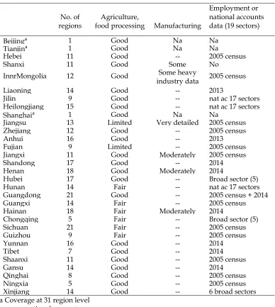
A key weakness relative to the Australian TERM (Wittwer and Horridge, 2010) and USAGE-TERM (Wittwer 2017a) databases is that census data are not highly disaggregated in the sectoral dimension. This means that such data are less specific in estimating regional activities in manufacturing and services sectors than is so for US and Australian census data. The available broad industry census employment numbers for China provide some measure of prefecture-level economic activity. At worst, this means that broad sector outputs (outside of agriculture, for which data are sufficient) are split between the disaggregated sectors of the national database in identical proportions across all prefectures in a given province. In addition, available census data in a number of provinces are only for 2005.

Clearly, relatively recent employment data are preferable to 2005 census data. The 2005 data were used to estimate prefectural shares in Hebei, Inner Mongolia, Jiangsu, Zhejiang, Fujian, Jiangxi, Guangxi, Sichuan, Guizhou, Shaanxi, Qinghai and Ningxia. Employment data for prefectures by national accounts level (19 sectors) were available for either 2013 or 2014 in Liaoning, Anhui, Shandong, Henan, Hainan, Yunnan, Tibet and Gansu. The yearbooks of Jilin, Heilongjiang, and Hunan include 2014 national accounts (GDP) data for 17 broad sectors. Guangdong’s 2005 employment census data are supplemented by 2014 GDP data for 9 broad sectors. Regions other than Hubei with limited data include Chongqing (divided into five main regions) and Xinjiang.

For some commodities, we were able to improve on yearbook data. For example, the Liaoning province yearbooks includes employment for a single manufactures sector. An online search indicates that within Liaoning, only Dalian and Shenyang produce motor vehicles, so activities for this sector in other prefectures within the province are set to zero. Prefectural level data are also available for meat products. But in remaining manufactures, the broad manufacturing employment shares provide the sub-provincial split.

14

Table 1. Summary of prefecture-level data quality

No. of

regions food processing Manufacturing Agriculture,

Employment or national accounts data (19 sectors)

Beijinga _{1 Good Na Na}

Tianjina _{1 Good Na Na}

Hebei 11 Good -- 2005 census

Shanxi 11 Good Some No

InnrMongolia 12 Good _{industry data} Some heavy 2005 census

Liaoning 14 Good -- 2013

Jilin 9 Good -- nat ac 17 sectors

Heilongjiang 15 Good -- nat ac 17 sectors

Shanghaia _{1 Good Na Na}

Jiangsu 13 Limited Very detailed 2005 census

Zhejiang 12 Good -- 2005 census

Anhui 16 Good -- 2013

Fujian 9 Limited -- 2005 census

Jiangxi 11 Good Moderately 2005 census

Shandong 17 Good -- 2014

Henan 18 Good Moderately 2014

Hubei 17 Good -- Broad sector (5)

Hunan 14 Fair -- nat ac 17 sectors

Guangdong 21 Good -- 2005 census + 2014

Guangxi 14 Fair -- 2005 census

Hainan 18 Fair Moderately 2014

Chongqing 5 Fair -- Broad sector (5)

Sichuan 21 Fair -- 2005 census

Guizhou 9 Fair -- 2005 census

Yunnan 16 Good -- 2014

Tibet 7 Good -- 2014

Shaanxi 11 Good -- 2005 census

Gansu 14 Good -- 2014

Qinghai 8 Good -- 2005 census

Ningxia 5 Good -- 2005 census

Xinjiang 14 Good -- 6 broad sectors

a Coverage at 31 region level nat ac = national accounts Na = not applicable

15

prefecture level gleaned from the province’s yearbooks are national accounts data for four broad non-agricultural sectors.

Regional household and government spending shares are based on expenditure-side macro accounts from the provincial statistical yearbooks. We assume that the commodity composition of household spending is the same across all regions. More specific data would enable us to alter these shares, based on

differences that may arise, for example, from climatic differences across regions.2

Another obvious weakness in the initial provincial-level database generated is that international trade activities in the database are calculated from available information on port activities rather than customs data. As with the first version

of TERM for Australia (Horridge et al., 2005), we expect initial international trade

by port estimates to be superseded by actual customs data.

In summary, there are two broad approaches to maintaining and improving the regional database. The first is that collaboration with model users will improve our access to actual data, in particular for international merchandise trade. The second is that the TERM suite of programs, referenced earlier in this section, enables us to generate a new database rapidly as better data emerge.

2.5 The TRADE matrix

The next stage is to construct a TRADE matrix. For each commodity either domestic or imported, TRADE contains a 365x365 submatrix, where rows correspond to region of origin and columns correspond to region of use. Diagonal elements show production that is locally consumed. We already know from regional shares used to split the national database both the row totals (supply by commodity and region) and the column totals (demand by commodity and region) of these submatrices. We use the gravity formula (trade volumes follow an inverse power of distance) to construct trade matrices consistent with pre-determined row and column totals. In defence of this procedure, note that wherever production (or, more rarely, consumption) of a particular commodity is concentrated in one or a few regions, the gravity hypothesis is called upon to do very little work. Because our sectoral classification is so detailed, this situation occurs more frequently than with a relatively aggregated sectoral dimension.

2 _{The Australian Bureau of Statistics produces the Household Expenditure Survey (HES), which}

16

The usual TERM gravity formula, as described in Horridge (2011) is:

r,d

k r,d

r,

,d

V

V

V

D

•

•

∝

r

≠

d

(1)

where

Vr,d = value of flow from origin r to destination d

Vr,• = production in r

V •,d = demand in d

Dr,d = distance from r to d

where K is a commodity-specific parameter valued between 0.5 and 2, with higher values for commodities not readily tradable.

Diagonal cells of the trade matrices are set according to:

d,d

d, V

V • = locally-supplied demand in d as share of local production

=

,d

V

min

,1 F

V

•





















(2)

where Fis a commodity-specific parameter valued between 0.5 and 1, with a

value close to 1 if the commodity is not readily tradable.

The initial estimates of V(r,d) are then scaled (using a RAS procedure) so that:

Σ

V(r,d)= V(

,d)

Σ

V(r,d)= V(r,

).

Transport costs as a share of trade flows are set to increase with distance:

T(r,d)/V(r,d)

∝

D(r,d)

where T(r,d) corresponds is a matrix or margins on the TRADE matrix (TRADMAR in Section 3, Table 11). Again, the constant of proportionality is chosen to satisfy constraints derived from the initial national IO table.

All these estimates are made with the fully-disaggregated database. In many

cases, zero trade flows can be known a priori. For example, tea is grown in a limited

number of prefectures in which the climate is suitable. At a maximum sectoral disaggregation, the load born by gravity assumptions is minimized.

2.6 Aggregation

17

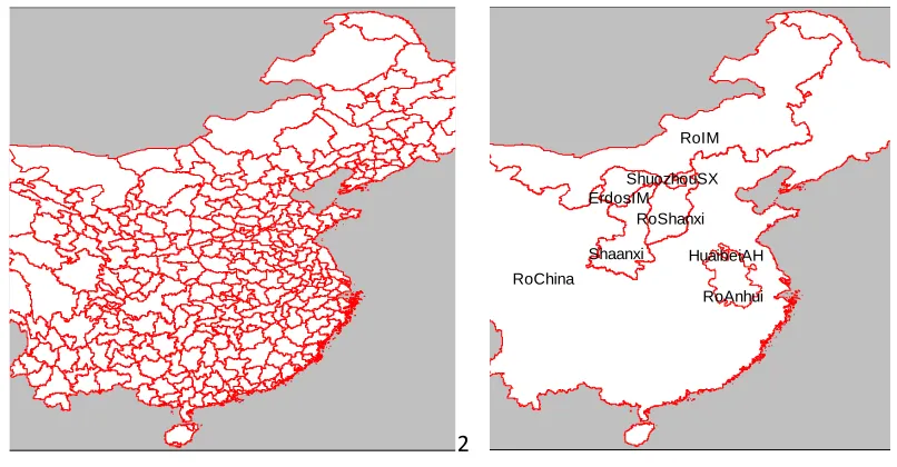
aggregation example is that of the simulation presented in section 5. This concerns a switch away from coal use in industries and in electricity generation. The sectoral aggregation preserves the coal mining sector, coal-generated electricity, hydro-electric generation and hydro-electricity distribution from the master database, while aggregating other sectors. There are 21 sectors in the aggregation.

In the regional dimension, three prefectures in which coal accounts for a large share of regional GDP are represented individually. These are Erdos (Inner Mongolia), Shuoxhou (Shanxi) and Huaibei (Anhui). In each case, a regional

composite covers the rest of the province. A 7th _{region is Shaanxi, in which coal}

accounts for a significant share of provincial GDP, and an 8th region the rest of

China. The 365 regions of the master database are aggregated to 8 regions (Figure 1).

1 2

Figure 1. Aggregating from master database to policy simulation regions

3

3. The equations of TERM 4

This section elaborates the core theory of the TERM suite of models. The format

5

of this section is to present the levels version of each block of equations. The model

6

is implemented using GEMPACK software (Harrison et al., 2014). TABLO coding

7

of the model’s equations follows each block. Within GEMPACK, most equations

8

are presented in a linearized form. Multi-step solution methods (Dixon et al., 1982,

9

chapter 5) enable the modeler to combine the accuracy of the levels form with the

10

relative simplicity and computational speed of linearized equations.

11

3.1 Production 12

RoChina

RoIM

Shaanxi RoShanxi

RoAnhui ErdosIM

ShuozhouSX

18

Each industry uses a combination of intermediate and primary inputs to

13

produce a unit of output. Producer decisions consist of a sequence of CES

14

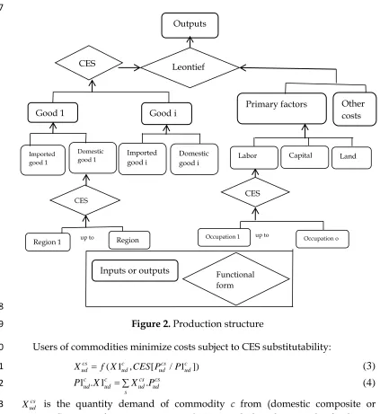
decisions, with a composite good entering the next stage. Figure 2 shows the

15

production structure.

16 17

18

Figure 2. Production structure

19

Users of commodities minimize costs subject to CES substitutability:

20

( 1 , [ / 1 ])

cs c cs c

ud ud ud ud

X = f X CES P P

(3)

21

1 . 1c_ud c_{ud ud}cs. _udcs s

P X = ∑X P

(4)

22

cs ud

X is the quantity demand of commodity c from (domestic composite or

23

imported) source s by user u in region d. Users include industries plus final users

24

(households, investors, exporters and government). cs

ud

P is the corresponding

25

Other costs Outputs

Good 1 Primary factors

Inputs or outputs Good i

CES _Leontief

Imported good 1

Domestic

good 1 Imported _{good i} Domestic _{good i} Labor Capital Land

CES

Region 1 up to Region

CES

Occupation o up to

Occupation 1

19

price, and X1c_ud and P1c_ud the respective domestic-import composite quantities and

26

prices.

27

Throughout the TABLO notation in this section, the index c refers to

28

commodities (COM), s to domestic or imported source (SRC), d to destination

29

(DST), u to users (USR) and i to industry (IND

∈

30

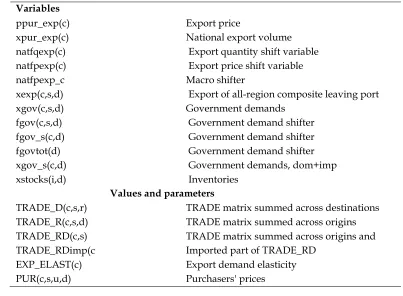
Table 2. Definitions of variables, values and parameters in intermediate and final usage

31

Variables

xint(c,s,i,d) Source-specific (dom./imp.) intermediate demands xint_s(c,i,d) Source-composite intermediate demands

xhou(c,s,d) Source-specific (dom./imp.) household demands xhou_s(c,d) Source-composite household demands

xinv(c,s,d) Source-specific (dom./imp.) investment demands xinv_s(c,d) Source-composite investment demands

ppur(c,s,i,d) Source-specific (dom./imp.) tax-inclusive com. price for user ppur_s(c,i,d) Source-composite tax-inclusive commodity price for user puse(c,s,u,d) Source-specific (dom./imp.) commodity price for user tuser(c,s,u,d) Powers of commodity taxes

pint(i,d) Intermediate effective price indices pinvest(c,d) Purchaser's price for investment phou(c,s,d) Household price

aint_s(c,i,d) Intermediate tech change

Values, shares and parameters

PUR_S(c,i,d) Purchasers' values summed over sources

PUR_CS(i,d) Purchasers' expenditure summed over commodities SIGMADOMIMP(c) CES parameter, domestic v. import sources

Listing 1 shows the percentage change quantity equations concerning equation

32

(3) in TABLO format.3 The indexes “hou” and “inv” refer to the household and

33

investment elements of the user set.

34

Listing 1. Intermediate and final usage (partial TABLO coding)

35

xint(c,s,i,d) = xint_s(c,i,d) -

SIGMADOMIMP(c)*[ppur(c,s,i,d)-ppur_s(c,i,d)]; (T3a)

xhou(c,s,d) = xhou_s(c,d) -

SIGMADOMIMP(c)*[ppur(c,s,"hou",d)-phou(c,d)]; (T3b)

3Note that the TABLO equation numbering follows that of previous equations in text: i.e.,

20

xinv(c,s,d) = xinv_s(c,d) -

SIGMADOMIMP(c)*[ppur(c,s,"inv",d)-pinvest(c,d)]; (T3c)

ppur(c,s,u,d) = puse(c,s,d) + tuser(c,s,u,d); (T4a)

PUR_CS(i,d))*pint(i,d)=

sum{c,COM,PUR_S(c,i,d)*[ppur_s(c,i,d)+aint_s(c,i,d)]}; (T4b)

pinvest(c,d) = ppur_s(c,"Inv",d); (T4c)

phou(c,d) = ppur_s(c,"hou",d); (T4d)

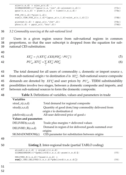
3.2 Commodity sourcing at the sub-national level 36

Users in a given region source from sub-national regions in common

37

proportions, so that the user subscript is dropped from the equation for

sub-38

national CES substitution:

39 40

( 1 , [ / ]

cs cs cs cs

rd d rd d

XT = f XT CES PD PU

(5)

41

. 1 .

c cs cs cs

sd d rd rd

r

PU XT = ∑XT PD

(6)

42

The total demand for all users of commodity c, domestic or import source s,

43

from sub-national origin r to destination d is cs

rd

XT . Sub-national source composite

44

demands are denoted by XT1cs_d and user prices by PU_sdc . TERM substitutability

45

possibilities involve two stages, between a domestic composite and imports, and

46

between sub-national sources to form the domestic composite.

47

Table 3. Definitions of variables, values and parameters in trade

48

Variables

xtrad_r(c,s,d) Total demand for regional composite

xtrad(c,s,r,d) Quantity of good dom/imp commodity delivered from origin r to destination d

pdelivrd(c,s,r,d) All-user delivered price of good c

Values and parameters

DELIVRD(c,s,r,d) Trade plus margins = delivered values

DELIVRD_R(c,s,d) Demand in region d for delivered goods summed over origins

SIGMADOMDOM(c) CES parameter for substitution between origins

49

Listing 2. Inter-regional trade (partial TABLO coding)

50

xtrad(c,s,r,d) = xtrad_r(c,s,d)

SIGMADOMDOM(c)*[pdelivrd(c,s,r,d)-puse(c,s,d)]; (T5)

DELIVRD_R(c,s,d))*puse(c,s,d) =

sum{r,ORG,DELIVRD(c,s,r,d)*pdelivrd(c,s,r,d)}; (T6)

21

Table 4. Definitions of variables, values and parameters in primary factor

53

demands

54

Variables

xlab(i,o,d) Labour demands, occupation specific plab(i,o,d) Wage rates, occupation specific xcap(i,d) Capital usage

xlnd(i,d) Land usage

pcap(i,d) Rental price of capital plnd(i,d) Rental price of land plab_o(i,d) Price of labour composite xlab_o(i,d) Effective labour input wlab_o(i,d) Wage bills

alab_o(i,d) Labor-augmenting technical change acap(i,d) Capital-augmenting technical change alnd(i,d) Land-augmenting technical change xprim(i,d) Primary factor composite

pprim(i,d) Effective price of primary factor composite Values and parameters

LAB(i,o,d) Wage matrix CAP(i,d) Rentals to capital LND(i,d) Rentals to land

LAB_O(i,d) Total labour bill in industry i PRIM(i,d) Total factor input to industry i SIGMAPRIM(i) CES parameter, primary factors

Next, we outline cost minimizing behaviour in primary factor demands by

55

industry users. The occupation o mix of labour follows a CES form:

56

( 1 , [ / 1 ])

o o

id id id id

L = f L CES W W (7)

57

1 . 1_{id id} o_id. _ido o

W L = ∑L W (8)

58

Occupation-specific labor demands are o

id

L and labour composite demands

59 1_id

L , with the corresponding wages being W_ido and W1_id.

60

1_id ( _id, [ 1 /_{id id}])

L = f F CES W PF (9)

61

( , ( / ])

id id id id

LND = f F CES RLND PF (10)

62

( , ( / ])

id id id id

K = f F CES R PF (11)

63

. . 1 . 1 .

id id id id id id id id

PF F =LND RLND +L W +K R (12)

22

Equations (9) to (12) show primary factor demands for the labour composite

65

L1id, capital Kid and land LNDid subject to a composite factor demand Fid by

66

industry i in region d. The factor prices are W1id for composite labour, Rid for

67

capital rentals, RLNDid for land rentals and PFid for composite prices.

68

Listing 3. Primary factor demands (partial TABLO coding)

69

xlab(i,o,d) = xlab_o(i,d) –

SIGMALAB(i)*[plab(i,o,d) - plab_o(i,d)]; (T5)

LAB_O(i,d))*wlab_o(i,d) =

sum{o,OCC,LAB(i,o,d)*[plab(i,o,d)+xlab(i,o,d)]}; (T6a)

LAB_O(i,d))*plab_o(i,d)=sum{o,OCC, LAB(i,o,d)*plab(i,o,d)}; (T6b)

xlab_o(i,d) - alab_o(i,d) = xprim(i,d) -

SIGMAPRIM(i)*[plab_o(i,d) + alab_o(i,d) - pprim(i,d)]; (T7)

xlnd(i,d) - alnd(i,d) = xprim(i,d) -

SIGMAPRIM(i)*[plnd(i,d) + alnd(i,d) - pprim(i,d)]; (T8)

xcap(i,d) - acap(i,d) = xprim(i,d) -

SIGMAPRIM(i)*[pcap(i,d) + acap(i,d) - pprim(i,d)]; (T11)

PRIM(i,d))*pprim(i,d) = LAB_O(i,d)*[plab_o(i,d) + alab_o(i,d)]

+ CAP(i,d)*[pcap(i,d) + acap(i,d)]

+ LND(i,d)*[plnd(i,d) + alnd(i,d)]; (T12)

70

The composite factor demand Fid is proportional to total output Qid subject to a

71

primary-factor using technology Aid.

72

. id id id

F =Q A (13)

73

The demand X1cid is related to output Qid by a CES relationship between the

74

composite price P1c_id and the price composite of all intermediate goods P11id via a

75

CES function.

76

1c_id ( _id, [ 1 / 11 ])c_{id id}

X = f Q CES P P (14)

77

11 . 11_{id id id}c. 1c_id c

P X = ∑P X (15)

78

The zero pure profit condition is that total revenue, valued at the output price net

79

of production taxes, PCid, multiplied by Qid equals the total production cost.

80

. c. 1c o. o . .

id id id id id id id id id id

c o

PC Q =∑P X +∑W L +R K +RLND LND (16)

23

Table 5. Definitions of variables and parameters in composite factor demands

83

Variables

xtot(i,d) Industry outputs

atot(i,d) All-input-augmenting technical change aint_s(c,i,d) Intermediate tech change

delPTX(i,d) Ordinary change in production tax revenue pcst(i,d) Ex-tax cost of production

ptot(i,d) Industry output prices

delPTXRATE(i,d) Change in rate of production tax

Values and parameters

SRCSHR(c,s,u,d) Imp/dom shares VCST(i,d) Total cost of industry i PRODTAX(i,d) Taxes on production

Next, we introduce production taxes to industry costs. Production tax revenue,

84

VPTXid, is calculated as the tax rate RPTXid multiplied by the value of output. The

85

industry output price PTOTid is inclusive of production taxes.

86

. .

id id id id

VPTX =RPTX PC Q (17)

87

. .[1 ].

id id id id id

PTOT Q =PC +RPTX Q (18)

88

Listing 4. Composite factor demands (partial TABLO coding)

89

xprim(i,d) = xtot(i,d)+atot(i,d)+aprim(i,d); (T13)

xint_s(c,i,d) = atot(i,d) + aint_s(c,i,d) + xtot(i,d)

-0.15*{ppur_s(c,i,d) + aint_s(c,i,d) - pint(i,d)}; (T14)

ppur_s(c,u,d)=sum{s,SRC,SRCSHR(c,s,u,d)*ppur(c,s,u,d)}; (T15)

VCST(i,d))*[pcst(i,d)-atot(i,d)] =

PRIM(i,d)*[aprim(i,d)+pprim(i,d)] + PUR_CS(i,d)*pint(i,d); (T16)

delPTX(i,d) =0.01*PRODTAX(i,d)*[xtot(i,d)+pcst(i,d)] +

VCST(i,d)*delPTXRATE(i,d); (T17)

VTOT(i,d))*[ptot(i,d)+xtot(i,d)]=

VCST(i,d)*[pcst(i,d)+ xtot(i,d)] + 100*delPTX(i,d); (T18)

In applications of the model in which industries have multi-product capability,

90

supplies of commodity c by industry i in region d (MQcid) follow a CET relationship

91

between industry output prices and the average commodity price PDOMcd, which

92

is the basic domestic price (see (50)).

93

( , ( / ])

cid id cd id

MQ = f Q CET PDOM PTOT (19)

94

.

id id cd cid

c

PTOT Q = ∑PDOM MQ (20)

95

We assume that the supply of imports is infinitely elastic. Hence, the price of

96

imports, PMcd, depends on foreign import prices, PFMcd and the nominal exchange

97

rate φ.

24 .

cd cd

PM =PFM φ (21)

99

Table 6. Definitions of variables and parameters in industry supplies

100

Variables

xmake(c,i,d) Output of good c by industry i in d pmake(c,i,d) Price received by industries

pdom(c,r) Output prices = basic prices of domestic goods xcom(c,d) Total output of commodities

Values and parameters

phi Exchange rate, local currency/$world pimp(c,r) Import prices, local currency

pfimp(c,r) Import prices, foreign currency

SIGMAOUT(i) Constant elasticity of transformation parameter

101

The TABLO coding for multi-product industries is:

102

Listing 5. Industry supplies (partial TABLO coding)

103

xmake(c,i,d)=xtot(i,d)+SIGMAOUT(i)*[pmake(c,i,d) ptot(i,d)]; (T19)

pmake(c,i,d)=pdom(c,d)-0.05*[xmake(c,i,d)-xcom(c,d)]; (T20)

pimp(c,r) = pfimp(c,r) + phi; (T21)

3.3 Household demands 104

The linear expenditure system (LES) is based on a utility function (U) which

105

splits household spending on each commodity (XHOUc) into two, a subsistence

106

component XSUBc that depends only on the number of households (N) and

107

preferences, and a luxury component, XLUXc, which depends on prices and

108

income in a Cobb-Douglas form.

β

109

spending minus aggregate subsistence spending) share of commodity c. Regional

110

and household dimensions are omitted from equations (22) to (33).

111

1

( ) c

c c

c

U XHOU XSUB

N

β

= Π − (22)

112

Aggregate spending (WHOU) is of the form:

113

[ ]

3c c 3c c 3c c

c c c

WHOU =ΣP XHOU =ΣP XSUB + WHOU−ΣP XSUB (23)

114

From this, we obtain the linear expenditure function, where P3c is the price faced

115

by household consumers of commodity c:

116

[ ]

3c c 3c c c 3d d

d

WHOU

P XHOU =P XSUB +β − ΣP XSUB (24)

25

Aggregate subsistence expenditure WSUB is given by:

118

3 ._{c c} c

WSUB= ∑P XSUB (25)

119

The Frisch “parameter” is the (negative) ratio of total expenditure to luxury

120

expenditure:

121

Frisch= -WHOU/[WHOU –WSUB] (26)

122

The ORANI school (Dixon et al., 1982) typically assigns a Frisch “parameter” of

123

-1.82 to a model for a relatively high income nation.

124

Differentiating equation (24) with respect to WHOU, and multiplying by

125

WHOU/[XHOUc.P3c], we calculate the expenditure elasticity EPSc. This is equal to

126

the marginal budget share divided by the budget share

127

(SHOUc=P3c.XHOUc/WHOU) for each commodity:

128

. / [ 3 . ]

c c c c

EPS =β WHOU P XHOU (27)

129

BLUXcis the ratio of luxury expenditure to total expenditure on each commodity,

130

given by:

131

[ ] / [ 3. ]

c cWHOU WSUB c c

BLUX =β − P XHOU (28)

132

Substituting equations (26) and (27) into equation (28):

133

/

c c

BLUX = −EPS Frisch (29)

134

Next, we calculate the matrix of price elasticities implied by LES. By

135

differentiating equation (24) with respect to P3d [i.e.,

136

/ 3 / 3

c d c d c

dXHOU dP = −β XSUB P ], we calculate the off-diagonal elements of the

137

price elasticity matrix (ηcd):

138

.[ ]

/ 3 3 /

c d d c

dXHOU dP P XHOU =

139

]

.( )( 3 )/( . 3 ).[ 3 /

c WHOU P XSUBd d WHOU P c P d XHOUc

β

− (30)

140

(1 ). /

cd c BLUXd SHOU SHOUd c

η =β − (31)

141

We obtain the diagonal elements by dividing equation (24) by P3c and

142

differentiating with respect to P3c:

143

.

/ 3 [ 3 / ]

c c c c

dXHOU dP P XHOU = −βcWHOU/[ 3P c.XHOUc ]+

144

. .

( ) 3 /[( . 3 ).[ 3 ]

cWHOU P dXSUBd WHOU P c P cXHOUc

β

Σ (32)

145

Substituting equations (27) and (31) into equation (32), we obtain:

26

cd d c

c

cc EPS

η η

≠

= − − ∑ (33)

147

LES does not allow for specific substitutability. Where appropriate, specific

148

substitutes could form a CES nest, with the CES composite commodity entering

149

LES within the model. In addition, LES does not allow for goods with negative

150

income elasticities.

151

SinoTERM365 includes provision for multiple households in each bottom-up

152

region. At present, there is only one household in the database in each region.

153

Individual households are denoted by h.

154

Table 7. Definitions of variables and shares in the household demand system

155

Variables

xhouh_s(c,d,h) Household demands

wlux(d,h) Total nominal supernumerary household expenditure xhouhtot(d,h) Total real household consumption

whouhtot(d,h) Total nominal household consumption phouhtot(d,h) CPI

nhouh(d,h) Number of households

xlux(c,d,h) Household - supernumerary demands xsub(c,d,h) Household - subsistence demands alux(c,d,h) Taste change, supernumerary demands asub(c,d,h) Taste change, subsistence demands

ahou_s(c,d,h) Taste change,household imp/dom compsite

Values and shares

BLUX(c,d,h) Luxury share of expenditure on commodity c BUDGSHR(c,d,h) Budget share

SLUX(c,d,h) Marginal budget share

Rather than include the general household demand equation in the model with

156

the elasticities implied by equations (31) and (33), the LES in SinoTERM365 is

157

coded as shown in Listing 5.

158

Listing 6. Household demand system (partial TABLO coding)

159

xlux(c,d,h) + phou(c,d) = wlux(d,h) + alux(c,d,h); (T24a)

xhouh_s(c,d,h)=BLUX(c,d,h)*xlux(c,d,h)+[1-BLUX(c,d,h)]*xsub(c,d,h)(T24b) alux(c,d,h) = asub(c,d,h) - sum{k,COM, SLUX(k,d,h)*asub(k,d,h)}; (T24d) asub(c,d,h)=ahou_s(c,d,h)-sum{k,COM,BUDGSHR(k,d,h)*ahou_s(k,d,h)};(T24e)

xsub(c,d,h) = nhouh(d,h) + asub(c,d,h); (T25)

27

A formula within the TABLO code calculates the share term BLUXc from

160

equation (29) and SLUXc based on equation (25). The Frisch “parameter” and

161

expenditure elasticities are updated as the subsistence share of consumption

162

changes. The usual practice has been to assign XSUBc as fixed. In modeling

163

relatively local changes, this is not an issue. But in dynamic modeling, particularly

164

when dealing with rapid income growth as in the case of the Chinese economy,

165

growing aggregate consumption results in XSUBc shrinking as a share of total

166

consumption of each commodity. This implies that the LES system tends towards

167

Cobb-Douglas as the economy grows over time. If this is unsatisfactory in a

168

particular scenario, the modeler may choose to increase per capita subsistence

169

consumption over time. This is justifiable on the basis that yesterday’s luxuries are

170

today’s necessities. An alternative functional form to LES that copes better with

171

growth in consumption over time is the AIDADS form, which also allows inferior

172

goods (Rimmer and Powell 1996).

173

To accommodate changes in per capita subsistence quantities, we may add to

174

SinoTERM365 an equation defining the percentage change in the Frisch

175

“parameter”, wfrisch:

176

wfrisch(d,h) = whoutot(d,h)-wlux(d,h); (T26)

177

A subsistence taste shifter asub_c is added to the following:

178

xsub(c,d,h) = nhou(d,h) + asub(c,d,h) + asub_c(d,h); (T24f)

179

alux(c,d,h) =asub(c,d,h) -asub_c(d,h)

180

-sum{k,COM, SLUX(k,d)*[asub(k,d,h)-asub_c(d,h)]}; (T24g)

181

In order to target a given shift in subsistence expenditures, the variable wfrisch is

182

made exogenous by swapping with asub_c.4

183

3.4 Investment demands 184

In the ORANI school, the commodity composition of investment varies

185

between industries. The amount of good c demanded by investment industry i in

186

region d, X2c_id, is proportional to the industry investment quantity, X2TOTid, for a

187

given investment technology A2c_id. P2cd is the commodity-specific investment

188

price.

189

2c_id 2 . 2c_{id id}

X =A X TOT (34)

190

4 _{In a dynamic simulation of an earlier SinoTERM version developed by the authors, aggregate}

28

, ,

2 . 2cd cd 1cInv d. 1cInv d

P X =P X Inv∈User (35)

191

,

2 . 2_{id id} 2 . 1c_id c_{Inv d} c

PI X TOT = ∑X P Inv∈User (36)

192

/ 2

id id id

GR =R PI (37)

193

Equation (34) calculates an industry investment price index. Equation (35) defines

194

the gross rate of return (GRid) as the ratio of the capital rental to the price of new

195

capital (i.e., the industry investment price index).

196

2 /

id id id

IKRAT =X TOT K (38)

197

2 0.33

[( ) / ]

id id

IKRAT = f GR Islack (39)

198

Equation (36) defines the investment-to-capital ratio (IKRATid). Typical, the gross

199

rate of return is exogenous in long-run simulations, with capital stocks (Kid)

200

endogenous – and the converse in the short run. Islack is exogenous except when

201

the simulation is accommodating a macro investment target. Equation (37) follows

202

the ORANI investment rule (Dixon et al. 1982). In dynamic applications of TERM,

203

the equations defining capital growth are replaced by a dynamic accumulation

204

equation linking present capital, past capital net of depreciation and past

205

investment (see Dixon and Rimmer, 2002, section 21).

206

Table 8: Definitions of variables and shares in investment demands

207

Variables

xinvitot(i,d) Investment by industry

pinvitot(i,d) Investment price index by industry

gret(i,d) Gross rate of return = Rental/[Price of new capital] ggro(i,d) Gross growth rate of capital = Investment/capital finv1(i,d) Investment shift variable

invslack Investment slack variable for exogenizing national investment fgret(i,d) Shifter to lock together industry rates of return

capslack Slack variable to allow fixing aggregate capital

Values

INVEST_I(c,d) Investment by commodity and region INVEST_C(i,d) Investment by industry and region

Listing 7. Investment demands (partial TABLO coding)

208

xinvi(c,i,d) = xinvitot(i,d); (T34)

INVEST_I(c,d)*xinv_s(c,d)= sum{i,IND,INVEST(c,i,d)*xinvi(c,i,d)}; (T35) INVEST_C(i,d)*pinvitot(i,d)= sum{c,COM,INVEST(c,i,d)*pinvest(c,d)}; (T36)

gret(i,d)= pcap(i,d) - pinvitot(i,d); (T37a)

gret(i,d) = fgret(i,d) + capslack; (T37b)

ggro(i,d)= xinvitot(i,d) - xcap(i,d); (T38)

29 3.5 Other final demands

209

Government demands XGcd are independent of prices and proportional to three

210

corresponding shifters. They shift the demand function with different dimensions:

211

by d as FGc, by c and d, as FGScd and by c, s, and d, as FGOVcsd.

212

. .

cd c cd csd

XG =FG FGS FGOV (40)

213

Export demands follow a two-stage process. First, regional source-specific exports

214

X4cd form a CES composite X4NATc:

215

4_cd ( 4 _c, [ 4_cd / 4 _c ])

X = f X NAT CES P P NAT (41)

216

,

4cd 1cExp d

P =P Exp∈User (42)

217

4 _c. 4 _c 4 . 4_{cd cd} d

P NAT X NAT = ∑X P (43)

218

Next, national exports are linked to international demands. FP4NATc and FQ4c are

219

demand shifters, and γ the export demand elasticity.

220

4 c ( 4 c / 4 c) 4c

X NAT = P NAT FP NAT −γFQ (44)

221 222

Inventories XSTid are proportional to XTOTid multiplied by a shifter, FSTid.

223

.

id id id

XST =Q FST (45)

30

Table 9: Definitions of variables and parameters in other final demands

226

Variables

ppur_exp(c) Export price

xpur_exp(c) National export volume

natfqexp(c) Export quantity shift variable natfpexp(c) Export price shift variable

natfpexp_c Macro shifter

xexp(c,s,d) Export of all-region composite leaving port

xgov(c,s,d) Government demands

fgov(c,s,d) Government demand shifter

fgov_s(c,d) Government demand shifter

fgovtot(d) Government demand shifter

xgov_s(c,d) Government demands, dom+imp

xstocks(i,d) Inventories

Values and parameters

TRADE_D(c,s,r) TRADE matrix summed across destinations TRADE_R(c,s,d) TRADE matrix summed across origins TRADE_RD(c,s) TRADE matrix summed across origins and

TRADE_RDimp(c Imported part of TRADE_RD

EXP_ELAST(c) Export demand elasticity

PUR(c,s,u,d) Purchasers' prices

Listing 8. Other final demands (partial TABLO coding)

227

xgov(c,s,d) = fgovtot(d) + fgov(c,s,d) + fgov_s(c,d); (T40a)

xgov_s(c,d) = sum{s,SRC, SRCSHR(c,s,"Gov",d)*xgov(c,s,d)}; (T40b)

xexp(c,"dom",d)=xpur_exp(c)-5*[ppur(c,"dom","Exp",d)-ppur_exp(c)]+ttradEXP(c,d); (T41)

ppur_exp(c)=Sum{d,Dst,PUR(c,"dom","exp",d)*[ppur(c,"dom","Exp",d)] (T43) xpur_exp(c) - natfqexp(c) = -EXP_ELAST(c)*

[ppur_exp(c)- phi - natfpexp(c) - natfpexp_c]; (T44)

xstocks(i,d) = xtot(i,d); (T45)

3.6 Margins 228

TERM separates the market for margins from the market for commodities being

229

delivered by margins m (Dixon et al., 1982). Demands for margins csm

rd

XTM are

230

proportional to commodity demands cs

rd

XT subject to a margins-using technology

231

csm rd

ATM (equation (46)).

232

.

csm csm cs

rd rd rd

XTM =ATM XT (46)

31

In equation (47), cs

r

PBAS is the basic commodity price and PM_rdm the margins’

234

prices. cs

d

PU is the margins-inclusive, tax-exclusive source-composite delivered

235

price that appears in equation (3.4).

236

. . .

cs cs cs cs m csm

rd rd r rd rd rd

m

PD XT =PBAS XT + ∑PM XTM (47)

237

. .

m m pm m

rd rd rd r

p

PMR XMR = ∑XMP PDOM (48)

238

( , [ / ])

pm m m m

rd rd r rd

XMP = f XMR CES PDOM PMR (49)

239

,

c dom

d cd

PBAS =PDOM (50)

240

,

c imp

d cd

PBAS =PIMP (51)

241

A third context is introduced for sub-national regions in equation (46). In

242

addition to regional origins r and destinations d for good and services, regions p

243

also produce margins. A shipping company that moves goods from origin in

244

Chongqing to a destination in Shanghai may be based in Wuhan (i.e., the margins

245

producing region). The Wuhan company competes with shipping companies from

246

other regions through CES substitution between regional providers p of margins

247

in equation (49). m

rd

PMR is the price of margins summed across providers p.

248

mp rd

XMP is the level of margins provided by p to move goods from region r to d

249

and m

rd

XMR the provider composite.

250

Table 10 contains the definition of variables, values and shares concerning

251

margins, followed by the TABLO coding.