Binarization of medical images based on the recursive application of mean shift filtering: Another algorithm

Binarization of medical images based on the

recursive application of mean shift

fi

ltering :

Another algorithm

Roberto Rodríguez

Digital Signal Processing Group, Institute of Cybernetics, Mathematics and Physics (ICIMAF), La Habana, Cuba

Correspondence: Roberto Rodriguez Digital Signal Processing Group, Institute of Cybernetics, Mathematics and Physics (ICIMAF), Calle 15 No. 551 e/C y D CP 10400, La Habana, Cuba

Email [email protected]

Abstract: Binarization is often recognized to be one of the most important steps in most high-level image analysis systems, particularly for object recognition. Its precise function-ing highly determines the performance of the entire system. Accordfunction-ing to many researchers, segmentation fi nishes when the observer’s goal is satisfi ed. Experience has shown that the most effective methods continue to be the iterative ones. However, a problem with these algorithms is the stopping criterion. In this work, entropy is used as the stopping criterion when segmenting an image by recursively applying mean shift fi ltering. Of this way, a new algorithm is introduced for the binarization of medical images, where the binarization is carried out after the segmented image was obtained. The good performance of the proposed method; that is, the good quality of the binarization, is illustrated with several experimental results. In this paper a comparison was carried out among the obtained results with this new algorithm with respect to another developed by the author and collaborators previously and also with Otsu’s method.

Keywords: image segmentation, mean shift, algorithm, entropy, Otsu’s method

Introduction

Nowadays, medical image breaking technologies have an enormous potential to con-tribute to the improvement of healthcare and medicine. Images have come to include not only diagnostic methods but also treatments by using image-guided methods. Healthcare is increasingly dependent not only upon the primary diagnostic technologies based on typical image visualization and analysis, but also on information, science, networking, image archiving and distribution, instrumentation, and treatment using physical energies.

A full understanding of image information is very important and image segmenta-tion, particularly binarizasegmenta-tion, plays an important role. Segmented images are now used routinely in a multitude of different applications, such as, diagnosis, treatment planning, localization of pathology, study of anatomical structure, and computer-integrated surgery. However, image segmentation, especially binarization, remains a diffi cult task due to both the variability of object shapes and the variation in image quality. Particularly, medical images are often corrupted by noise and sampling arti-facts, which can cause considerable diffi culties when applying rigid methods.

of complexity, shadows, and variability within and across individual objects. Furthermore, noise and other image arti-facts can cause incorrect regions or boundary discontinuities in objects recovered from these methods.

Today the most robust segmentation algorithms are the iterative methods, which cover a variety of techniques, rang-ing from the mathematical morphology, deformable models until the thresholding methods. However, one of the problems of these iterative techniques is the stopping criterion, where many methods have been proposed (Vincent and Soille 1991; Cheriet et al 1998; Chenyang et al 2000).

Mean shift is a nonparametric and versatile tool for feature analysis and can provide reliable solutions for many vision tasks (Comaniciu 2000; Comaniciu and Meer 2002). The mean shift was proposed by Fukunaga and Hostetler (1975) and largely forgotten until Cheng’s paper (1995) restored interest on it. Segmentation by means of the mean shift method carries out a smoothing fi lter as a fi rst step before segmentation is performed (Comaniciu 2000).

The term ‘entropy’ is not a new concept in the information theory fi eld. Entropy has been used in image restoration, edge detection, and recently as an objective evaluation method for image segmentation (Zhang et al 2003).

In this work, a new binarization strategy based on the computation of the mean shift is proposed. The proposal makes use of entropy as stopping criterion; of this way, binarization is easily obtained; that is, the binarization is carried out after the segmented image is attained. This is the main feature of the proposed algorithm; that is, to arrive to the segmented image directly from the fi ltering process and to carry out the binarization later.

The obtained results with this algorithm are compared with others developed by the author and collaborators and also with Otsu’s method (Rodríguez et al 2002a, 2003, 2005). In other words, our interest in this research is to determine which algorithm is the most suitable and robust for binariza-tion of medical images; in this case, blood vessels. In this work, the important information to be extracted from images is just the number of blood vessels present.

The remainder of the paper is organized as follows: In Theoretical aspects, we provide the more signifi cant theoretical aspects of the mean shift. In Entropy, we briefl y introduce the entropy concept. In Algorithms, we describe our binarization algorithm based on the mean shift by taking entropy as the stopping criterion. The experimental results, comparisons and discussion are presented. In this section a quantitative verifi cation of the obtained results is also carried out. Finally, the conclusions are exposed.

Theoretical aspects : The mean shift

The iterative procedure to compute the mean shift is intro-duced as a normalized density estimate of the gradient. By employing a differentiable kernel, an estimate of the density gradient can be defi ned as the gradient of the kernel density estimate; that is,

∇

( )

= ∇

( )

=

∑

∇

−

=

^ ^

f x

f x

nh

K

x

x

h

1

The kernel function K(x) is now a function, defi ned for

d-dimensional x, satisfying

K x dx

Rd ( ) =

∫

Other conditions on the kernel K(x) and the window radio

h are derived (Fukunaga and Hostetler 1975) to guarantee asymptotic unbiasedness, mean-square consistency, and uniform consistency of the estimate in expression (1). For example, for Epanechnikov kernel:

E

K x c d - xd if x

( ) 1/2 ( 2 ) 1 1

0

1 2

= − +

(

)

otherwise ⎧ ⎨ ⎪ ⎩⎪

where c_d is the volume of the unit d-dimensional sphere (Comaniciu 2000). The density gradient estimate becomes,

∇

=

⋅

_∑

−

=

⋅

f

x

x

x

x

E _{n h c}

d h

nx n h c

d h n d d d d x i xi Sh x

( )

(

)

(

2 ii

x

xi Sh x∈

∑

−

⎛ ⎝

⎜⎜ ( )

)

where the region S_h(x) is a hypersphere of radius h having volume hd c_d, centered at x, and containing n_x data points, that is, the uniform kernel. In addition, in this case d =3, for being the x vector of three dimensions, two for the spatial domain and one for the range domain (gray levels). The last term in expression (4) is called the sample mean shift.

M

x

n

x

x

n

x

x

h, U

x i

x i

xi Sh x xi Sh x

( )

1

(

)

The quantity _{nx n h}d c

d

( ) is the kernel density estimate

ˆ ( )

f_U x (where U means the uniform kernel ) computed with the hypersphere S_h(x), and thus we can write expression (4) as:

∇

=

⋅ +

f

x

x

d

h

M

x

E

( )

f

( )

( )

2

2

which yields,

M

x

h

d

f x

f

x

( )

( )

( )

= +

2

∇

^

^

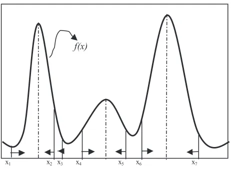
Expression (7) shows that an estimate of the normalized gradient can be obtained by computing the sample mean shift in a uniform kernel centered on x. In addition, the mean shift has the direction of the gradient of the density estimate at x when this estimate is obtained with the Epanechnikov

kernel. Since the mean shift vector always points towards the direction of the maximum increase in the density, it can defi ne a path leading to a local density maximum; that is, to a mode of the density (see Figure 1).

In addition, expression (7) shows that the mean is shifted towards the region in which the majority of the points reside. Since the mean shift is proportional to the local gradient estimate, it can defi ne a path leading to a stationary point of the estimated density, where these stationary points are the modes. Moreover, as it was pointed out the normalized gradient in expression (7) introduces a desirable adaptive behavior, since the mean shift step is large for low den-sity regions corresponding to valleys, and decreases as x

approaches a mode.

Mathematically speaking, this is justified since

∇^f x _{> ∇}^

f x E

E

U

f x

( )

( ) ( )

ˆ . Thus the corresponding step size for the

same gradient will be greater than that nearer mode. This will allow observations far from the mode or near a local minimum to move towards the mode faster than using

^

∇fE( )x alone.

Comaniciu and Meer (2002) proved that the mean shift procedure was obtained by successively:

• computing the mean shift vector M_h(x) • translating the window S_h(x) by M_h(x),

which guarantees convergence.

Therefore, if the individual mean shift procedure is guar-anteed to converge, a recursive procedure of the mean shift also converges. In other words, if one considers the recursive procedure to be like the individual sum of many procedures of the mean shift and each individual procedure converges, then the recursive procedure also converges. This claim was already proved by Grenier and colleagues (2006). The unanswered question is when to stop the recursive procedure. The answer is in the use of entropy as it will be shown in the next section.

A digital image can be represented as a two-dimensional array of p-dimensional vectors (pixels), where p =1 in the gray level case, p= 3 for color images, and p > 3 in the multispectral case.

As was pointed out by Comaniciu and Meer (2002), when the location and range vectors are concatenated in the joint spatial-range domain of dimension d = p +2, their different natures have to be compensated by proper normalization of parameters h_s and h_r. Thus, the multivariable kernel is defi ned as the product of two radially symmetric kernels and the Euclidean metric allows a single bandwidth for each domain, that is:

s h , rh

K x

C

s h

k xs

hs k xr hr ( ) 2 2 2 = ⎛ ⎝ ⎜ ⎞ ⎠ ⎟ ⎛ ⎝ ⎜ ⎞ ⎠ ⎟ r hp (8)

where xs _{is the spatial part, x}r _{is the range part of a feature} vector, k(x) the common profi le used in both domains, h_s and

h_r the employed kernel bandwidths, and C the corresponding normalization constant.

In this work all the segmentation experiments were per-formed by using a uniform kernel. In order for the comparison of the obtained results with both algorithms to be effective, the same parameters (h_r and h_s) were used. In this case, in all binarized images, h_s=12 and h_r=15, the uniform kernel was used. The value of h_s is related to the spatial resolution of the analysis while the value hr defi nes the range resolu-tion. It is necessary to note that the spatial resolution h_s has

x1 x2 x3 x4 x5 x6 x7

f(x)

a different effect on the output image when compared to the gray level resolution (h_r, spatial range). Only features with large spatial support are represented in the binarized image with our algorithm when h_s is increased. On the other hand, only features with high contrast survive when h_r is large. Therefore, the quality of segmentation and consequently binarization is controlled by the spatial value h_s and the range (gray level) h_r, resolution parameters defi ning the radii of the (3D/2D) windows in the respective domains.

Entropy

From the point of view of digital image processing the entropy of an image is defi ned as:

E X p X p X

X B

( )

( )

( )

= −

log₂

0 2 1

(9)

where B is the total quantity of bits of the digitized image and by agreement log₂(0) = 0; p(x) is the probability of occurrence of a gray-level value. Within a totally uniform region, entropy reaches the minimum value. Theoretically speaking, the prob-ability of occurrence of the gray-level value, within a uniform region is always one. In practice, when one works with real images the entropy value does not reach, in general, the zero value. This is due to existing noise in the image. Therefore, if we consider entropy as a measure of the disorder within a system, it could be used as a good stopping criterion for an iterative process, by using mean shift fi ltering. The entropy within each region diminishes in the measure that the regions become more homogeneous and at the same time in the whole image, until reaching a stable value. When convergence is reached, a totally segmented image is obtained, because the mean shift fi ltering is not idempotent, as it does not happen in mathematical morphology with some types of fi lters (for example, the opening fi lter is idempotent). In addition, as Comaniciu and Meer (2002) pointed out, the mean shift-based image segmentation procedure is a straightforward extension of the discontinuity preserving smoothing algo-rithm and the segmentation step does not add a signifi cant overhead to the fi ltering process.

The choice of entropy as a measure of goodness deserves several observations. First, it is known that the addition of two independent random variables (for example, a signal and additive noise) increases entropy (Zhang et al 2003). Entropy reduction reduces the randomness in corrupted probability density function and tries to counteract noise. Then, by fol-lowing this analysis, as the segmented image is a simplifi ed version of the original image, the entropy of the segmented

image should be smaller. Recently, it was empirically found that the entropy of the noise diminishes faster than that of the signal (Zhang et al 2003). Therefore, an effective criterion to stop would be when the relative rate of change of the entropy; from one iteration to the next, falls below a given threshold. This is the essential part of this work.

Algorithms

In this section two algorithms, one related with the fi ltering of the signal and the other related to the segmentation step are given.

Algorithm No. 1: Filtering algorithm

by using the mean shift

Let X_i and Z_i, i = 1,..,n, be the input and fi ltered images in the joint spatial-range domain. For each pixel p ∈ X_i, p=

(

)

( )

βbeing the quantity of bits/pixel in the image. The fi ltering algorithm comprises the following steps (Comaniciu 2000):

1. Initialize j =1 and y_i,1= p_i.

2. Compute through the mean shift (see expression (3),

y_{i, j+1}), the mode where the pixel converges; that is, the calculation of the mean shift is carried out until con-vergence, y = y_i,c.

3. Store at Z_i the component of the gray level of calculated value: Zi x yi

s i c

r

=

(

)

x

i, cr

y

Algorithm No. 2: Binarization algorithm

by recursively applying the mean shift

fi

ltering

Let ent1 be the initial value of the entropy of the fi rst itera-tion. Let ent2 be the second value of the entropy after the fi rst iteration. Let errabs be the absolute value of the difference of entropy between the fi rst one and the second iteration. Let

parlog be the parameter to carry out parametric logarithm. Let

edsEnt be the threshold to stop the iterations; that is, this is threshold to stop when the relative rate of change of the entropy; from one iteration to the next, falls below this threshold. Then, the segmentation algorithm comprises the following steps: 1. Initialize ent2 = 1, errabs = 1, edsEnt = 0.001. 2. While errabs > edsEnt, then

2.1. Filter the image according to the steps of the previous algorithm; store in Z [k] _{the fi ltered image.}

2.3. Calculate the absolute difference with the entropy value obtained in the previous step; errabs = /ent1 – ent2/.

2.4. Update the value of the parameter; ent2 = ent1;

Z[k +1]= _Z[k]_.

3. To carry out a parametric logarithm (parlog = 70). 4. Binarization: to assign to the background the white color

and to the objects the black color.

It is possible to observe that, in this case, the proposed segmentation algorithm is a direct extension of the fi ltering algorithm, which fi nishes when the entropy reaches the stability. Note the simplifi cation of this algorithm compared with the one proposed by Rodriguez and colleagues (2005) (see Algorithm steps in next section). Some comments on this algorithm follow. In (Christoudias et al 2002), it was stated that the recursive application of the mean shift property yields a simple mode detection procedure. The modes are the local maxima of the density. Therefore, with the new segmentation algorithm, by recursively applying mean shift, convergence is guaranteed. Indeed, the proposed algorithm is a straightforward extension of the fi ltering process. Comaniciu (2000) proved that the mean shift procedure converges. In other words, one can consider the new segmentation algorithm as a concatenated application of individual mean shift-fi ltering operations. Therefore, if we consider the whole event as linear, the recursive algorithm converges. Binarization is carried out after the segmented image is obtained.

Algorithm steps

The steps of the developed previously binarization algorithm are the following:

1. Run the mean shift-fi ltering procedure according to former steps, obtaining at Z the fi ltered image.

2. Defi ne the regions, which are found in the spatial domain

(hs) and that its intensities are smaller or equal than

hr/2.

3. For each region, which was defi ned in the step 2, one looks for all the pixels belonging to the patient and the mean of the intensity values are assigned at Z.

4. Build the region graph through an adjacent list of the following way: for each region, one looks for all adja-cent regions that are on the right hand side and below the patient.

5. While there exists nodes in the graph, which have been not visited, to run a variant of the depth-fi rst search (DFS), which concatenates adjacent regions, where we gave as parameter a node, which has been not visited. This according to steps following:

5.1 Mark the mentioned node as visited. 5.2 While children exist without visiting children = current child

if |Z_parent− Z_child|<= hr, then,

The region of the child is fused with the region of the father where the same label is assigned and it is marked as visited.

To the parent is assigned the visited child from the fi rst position and the children which have been not visited remain.

5.3 To look for the following child and come back to the step 2 while the stability has not yet been obtained (ie, no more pixel value modifi cations).

6. Eliminate spatial regions containing less than M pixels, since those regions are considered irrelevant.

7. (Binary): To all the pixels belonging to background, one assigns the white color and the black color to objects.

Experimental results : Analysis

and discussion

Evaluation method

Manual segmentation generally gives the best and most reliable results when identifying structures for a particular clinical task. Up to now and due to the lack of ground truth, the quantitative evaluation of a binarization method is dif-fi cult to achieve. An alternative is to use manual-binarization results as the ground truth.

In order to evaluate the performance of both techniques, we calculated the percentage of false negatives (FN; objects that are not found by the strategy) and the false positives (FP; noise, which is classifi ed as objects). These were defi ned according to the following expressions,

FP f p

Vp f p

FN fn

Vp fn

= +

= +

*

* 100

100

(10)

where Vp is the actual number quantity of objects identifi ed by the physician, f_n being the quantity of objects, which were not marked by the strategy and f_p being the number of spuri-ous regions, which were marked as objects.

Experimental results

a piecewise constant model is enforced over the image. In this work, after the segmented image was obtained based on the recursively application of mean shift fi ltering, a binarization procedure was carried out according to algorithm No. 2.

Some details on the original images are given next. Studied images are biopsies, which represent an angiogenesis process in malignant tumors. These were included in paraffi n by using the inmunohistoquimic technique with the complex method of avidina biotina. Finally, monoclonal CD34 was contrasted with green methyl to accentuate formation of new blood vessels. These biopsies were obtained from soft parts of human bodies. This analysis was carried out for more than 80 patients. These images were captured via MADIP system with a resolution of 512 × 512 × 8 bit/pixels (Rodríguez et al 2001).

There are several notable characteristics of these images, which are common to typical images that we encounter in the tissues of biopsies:

1. The intensity is slightly darker within the blood vessel than in the local surrounding background. It is empha-sized that this observation holds only within the local surroundings.

2. High local variation of intensity is observed both within the blood vessel and the background. However, the local variation of intensity is higher within the blood vessel than in background regions.

3. The variability of blood vessels both, in size and shape can be observed.

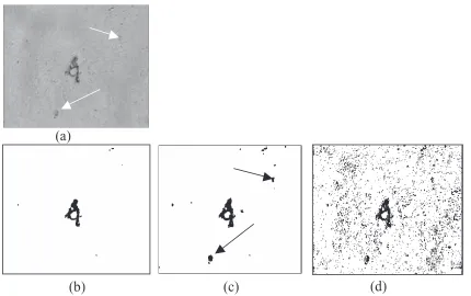
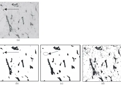
A first segmentation example carried out with both algorithms is shown in Figure 1. Although Otsu’s method was already applied in a previous work (Rodríguez et al 2002b), one can observe the obtained result by using this technique.

We note in Figure 1 that the binarized image using the new algorithm was cleaner and it didn't accentuate the spurious information that appears in the original image (see arrows in Figure 1a). According to criterion of pathologists these objects (spurious, with little contrast) were originated by a problem in the preparation of the samples. The obtained result by using Otsu’s method is evident. One can observe the spurious information. This best result with the new binarization algorithm is because the same one is a direct extension of the fi ltering process and therefore this algorithm did not make mistakes. The parameter used to carry out the parametric logarithm was similar to 70 and this value was the same for all the binarized images. In the experimentation was proven that the fi nal result is not very sensitive to this parameter, because a variation in the range from 40 to 70 led to the same result. The obtained results can be observed with the new algorithm and those attained by Rodríguez and colleagues (2002b, 2003). We see in Figure 2 that entropy

(a)

(b)

(c)

(d)

diminishes in iteration by iteration until reaching a stable value, that is, until convergence.

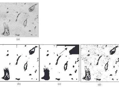
After the convergence was reached, a binarization procedure was carried out (see Algorithm No. 2). Another segmentation example carried out with both algorithms is shown in Figure 3.

It is evident to observe that the binarized image by using the new algorithm has a better appearance than the obtained image by using graph. Note, in this case, that the binariza-tion algorithm by using graph made a mistake (see arrow in Figure 3c). In practice, it has been proven that this behavior did not always happen with all images and in the corners of the images this was manifested fundamentally. This was what motivated us to look for a more effi cient algorithm, which this paper proposes. We see that the structures binarized with the new algorithm (see Figure 3b) are more similar to the original (see interior part of the blood vessels). On the other hand, the binarized image using Otsu’s method was better than in Figure 1d, but the image was still very noisy. This result is not good according to the physicians’ criterion, since these images will be subject to a further morphometrical analysis in order to diagnose and prognosticate malign tumors automatically.

In many occasions, given the application, binarization imposes certain conditions (elimination of regions, pruning or integration of certain maxima, etc). This can originate a biased image with regards to the initial image. With the new algorithm the resolution is only imposed on the segmentation process; that is, to parameters h_r and h_s. For this reason, the new algorithm did not make mistakes; that is, a binarized image very differ-ent to the original was never obtained. This is one of the most important experimental results obtained with the new algorithm.

No. Iterations E

N T R O P Y y

Threshold

1 2 3 4 5 6 7 8 9

2.7928

Figure 2 Decrease of the entropy in each one of the iterations.

(a)

(b) (c) _(d)

Observe the obtained results with the new algorithm and those attained by Rodríguez and colleagues (2002b, 2003).

From Figure 4, we observe that, iteration by iteration, the convergence was reached. After this step, binarization was carried out.

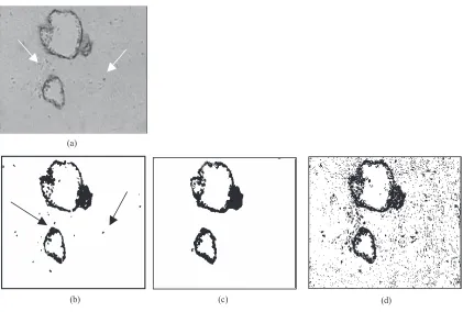
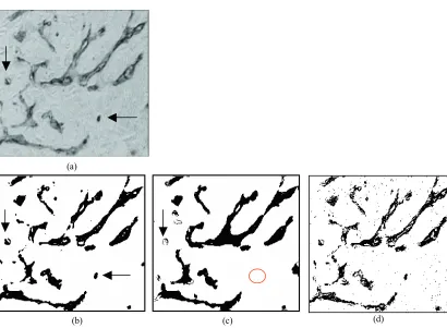
In Figure 5, another example of segmentation carried out with both algorithms is shown.

The difference among the three results is observed. Although, apparently, the result of the new algorithm is noisier,

according to criterion of the physicians’ criterion, the result of Figure 5b is correct. In the case of the obtained result with the algorithm by using graph, some objects (blood vessels) were eliminated, which lost important information (see arrows in original image). This behavior is due to parameter M, which has as a goal to eliminate the areas or irrelevant objects. It is not necessary to use this parameter with the new algorithm (see Algorithms). The result obtained with Otsu’s method is very noisy. In our previous research (Rodriguez et al 2002b), we proposed a variant in order to work with Otsu’s method. If one carries out a morphological fi lter (for example, an open-ing) after the obtained result by using Otsu’s method, many objects (blood vessels) can be eliminated. This happened even when one selected the most appropriate structure element. We confi rmed this in a previous work (Rodríguez et al 2003).

As a last example, the behavior of the entropy until the algorithm reaches convergence can be appreciated (Figure 6). Other examples appear in Figures 7, 8, and 9.

In the last examples, the most signifi cant differences in the obtained results with both algorithms can be observed in the images of Figures 7 and 9 with arrows shown. The differences in both algorithms with respect to Otsu’s method are evident. Otsu’s method originated a lot of noise in all cases. It was proven that even when the images were fi ltered with Gauss, the results obtained with Otsu’s method were

No. Iterations E

N T R O P Y y

Threshold

1 2 3 4 5 6 7 8 9

2.4565

Figure 4 Decrease of the entropy in each one of the iterations. It is interesting to observe that in the iteration 4 an increase of the entropy is noticed, but starting from this iteration the entropy falls quickly.

(a)

(b) (c) (d)

not good. The best result obtained by using the mean shift algorithm is because the mean shift is a good low pass fi lter. On the other hand, the obtained result in Figure 7 with the algorithm that uses graph, at least, an object was eliminated (see circle in Figure 7c). This issue, as in previous images was explained as caused by the parameter, M. Please note that this did not happen to the binarized image obtained with the new algorithm (see Figure 7b). In Figure 9, the obtained result with the new algorithm is verifi ed as being more robust. Observe that, on one hand, the binarized objects are more

contrasted (see vertical left arrows in Figures 9b, 9c), and that on the other hand, with the algorithm that uses graph, at least, a blood vessel was eliminated (see circle in Figure 9c).

As it was pointed out earlier, the important information to be extracted from images in this work is just the number of blood vessels present. These images will be subject to a morphometrical analysis in order to diagnose automatically and predict malignant tumors based on the numbers of blood vessels in a certain area. In this case the size of blood vessels is not important.

Quantitative comparison among

all algorithms

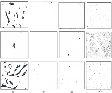
Since much of the motivation for biomedical image binariza-tion is to automate all or part of the binarizabinariza-tion process, it is perhaps more important to compare the results obtained by automatic binarization against those obtained by manual binarization. In Figure 10, three examples of the calculated XOR among the manual binarization and binarization by using both graph and new algorithm and also Otsu’s method are shown. In this validation only three of the analyzed images were presented; nevertheless, this comparison was carried out with all images.

Results reported in this investigation have been confi rmed by qualitative and quantitative comparisons by pathologists

No. Iterations E

N T R O P Y y

Threshold

1 2 3 4 5 6 7 8 9

3.618

Figure 6 Behavior of the entropy until the algorithm reaches the convergence.

(a)

(b) (c) (d)

(a)

(b) (c) (d)

Figure 8 (a) Original image. (b) Binarized image by using the new algorithm. (c) Binarized image by using graph. (d) Binarized image via Otsu’s method.

(a)

(b) (c) (d)

because they know the objects that they want to isolate. Therefore, in order to evaluate the performance of all algorithms, the percentage of false positives and false negatives was calculated among the result from the binarization and from the manual binarization. Numerical results of the comparison, by using the expression (10), were summarized in Table 1 (binarization obtained by recursively applying the mean shift fi ltering), Table 2 (binarization obtained by using graph), and Table 3 (binarization obtained via Otsu’s method).

In Table 1, the case of recursively applying the mean shift fi ltering showed that the percent error for false negatives were equal to 0%; that is, all regions belonging to blood vessels were detected. This denoted the correct performance of the new algorithm. This behavior was the same for the 80 bina-rized images. However, in Table 2, it is possible to note that with the algorithm that appears in the Algorithm steps section (by using graph), in two occasions the FN was different of cero; that is, the algorithm was not able to detect all the blood vessels. This issue happened with other binarized images.

This is due to the aggressiveness of the parameter M in the algorithm of the Algorithm steps section. Therefore, this parameter (M) should be set to a small value for this applica-tion type; otherwise the diagnosis can be erroneous. In Table 3, one can see that Otsu’s method did not originate FN; that is, all objects (blood vessels) were detected. However, Otsu’s method originated a lot of FP, which was related with the noise it created. This proves the advantage of the new algo-rithm with regard to the previous one because, besides being simpler, this doesn't use the parameter, M. Nevertheless, the

(a) (b) (c) (d)

Figure 10 (a) Manual binarization images. (b) XOR with the binarized images by recursively applying the mean shift fi ltering. (c) XOR with the binarized images by using graph. (d) XOR with the binarized images via Otsu’s method (see Figures 1, 7, and 9).

Table 1 Numerical results of comparison between manual and automatic binarization (by recursively applying the mean shift fi ltering)

Images V_p f_p f_n FN FP

algorithms that used the mean shift were superior, in this application, to Otsu’s method.

In Figures 10b and 10c it can be noted that the binarization process was not completely correct. It can be seen, according to the judgment of physicians, which some false positives arose. However, in all the cases for both algorithms, the FP was less than 15%. The obtained results (FP) by using Otsu’s method were previously explained and these were not good.

The false positives may arise due to transition of illumination or a change of contrast in the preparation of the samples. In practice, these problems are very diffi cult to eliminate completely in real images. Then, the result from the full automatic binarization steps was presented to the physicians. With a few mouse clicks on the fi nal result, the false positives were completely eliminated.

Conclusions

We propose a new algorithm that applies recursively the mean shift fi ltering and uses entropy as the stopping criterion. With this new algorithm the binarization was carried out after the image was segmented. Starting from the obtained results, working with real images, we demon-strated that the new binarization algorithm through recursive application of the mean shift was more effective and more robust than the algorithm using graph. Also, it was shown that the binarized images with the new algorithm were always the correct ones; that is, this algorithm did not made a mistake. It was proven that, in all cases, the new algorithm was superior to Otsu’s method. This new algorithm can be applied to other types of images and it can be extended to other tasks of analysis of images where robust methods of binarization are required.

Disclosure

The author has no confl ict of interest in this work.

References

Cheng Y. 1995. Mean shift, mode seeking, and clustering. IEEE Trans Pattern Anal Mach Intell, 17:790–9.

Chenyang X, Dzung P, Jerry P. 2000. Image segmentation using deformable models. In: Fitzpatrick JM, Sonka M (eds). SPIE Handbook on Medical Imaging, Medical Image Analysis. Vol. III, pp. 129–74.

Cheriet M, Said JN, Suen CY. 1998. A recursive thresholding technique for image segmentation. IEEE Trans Image Proc, 7:918–21.

Chin-Hsing C, Lee J, Wang J, et al. 1998. Color image segmentation for bladder cancer diagnosis. Mathl Comput Modeling, 27:103–20. Christoudias CM, Georgescu B, Meer P. 2002. Synergism in low level

vision. 16th International Conference on Pattern Recognition, Quebec City, Canada, August 2002, 4:150–5.

Comaniciu D, Meer P. 2002. Mean shift: A robust approach toward feature space analysis. IEEE Trans Pattern Anal Mach Intell, 24:603–19. Comaniciu DI. 2000. Nonparametric robust method for computer vision.

Ph.D. Thesis, New Brunswick, Rutgers: The State University of New Jersey.

Fukunaga K, Hostetler LD. 1975. The estimation of the gradient of a density function. IEEE Trans Info Theory, 21:32–40.

Grenier T, Revol-Muller C, Davignon F, et al. 2006. Hybrid approach for multiparametric mean shift fi ltering. Image Processing, 2006 IEEE, International Conference, Atlanta, GA, Oct 8–11, 2006. pp. 1541–4. Koss JE, Newman FD, Johnson TK, et al. 1999. Abdominal organ

segmen-tation using texture transforms and a Hopfi eld neural network. IEEE Trans Med Imaging, 18:640–8.

Rodríguez R, Alarcón TE, Abad JJ. 2003. Blood vessel segmenta-tion via neural network in histological images. J Intell Robot Sys, 36:451–65.

Rodríguez R, Alarcón TE, Castillo I. 2002a. A strategy for reduction of noise in segmented images. Its use in the study of angiogenesis. J Intell Robot Sys, 33:99–112.

Rodríguez R, Alarcón TE, Sánchez TL. 2001. MADIP: Morphometrical analysis by digital image processing. Proceedings of the IX Spanish Symposium on Pattern Recognition and Image Analysis. I:291–8. Rodríguez R, Alarcón TE, Wong R, et al. 2002b. Color segmentation applied

to study of the angiogenesis. J Intell Robot Sys, 34:83–97.

Rodríguez R, Suárez AG, Castillo PJ. 2005. [Utilización de la media desplaza para la segmentación de imagines] In Spanish. Boletín de la Sociedad Cubana de Matemática y Computación, 3:1.

Schmid P. 1999. Segmentation of digitized dermatoscopic images by two-dimensional color clustering. IEEE Trans Med Imaging, 18:164–71. Shareef N, Wang DL, Yagel R. 1999. Segmentation of medical images using

LEGION. IEEE Trans Med Imaging, 18:74–91.

Sijbers J, Scheunders P, Verhoye M, et al. 1997. Watershed-based segmen-tation of 3D MR data for volume quatization. Magn Reson Imaging, 15:679–88.

Vincent L, Soille P. 1991. Watersheds in digital spaces: An effi cient algorithm based on immersion simulations. IEEE Trans Pattern Anal Mach Intell, 13:583–98.

Wu K, Gauthier D, Levine MD. 1995. Live cell image segmentation. IEEE Trans Biomed Eng, 42:1–12.

Zhang H, Fritts JE, Goldman SA. 2003. An entropy-based objective evalua-tion method for image segmentaevalua-tion. In: Yeung M, Lienhart M, Rainer W, et al. (eds). Storage and Retrieval Methods and Applications for Multimedia 2004. Proceedings of The SPIE, 5307:38–49.

Table 2 Numerical results of comparison between manual and automatic binarization (by using graph)

Images Vp fp fn FN FP

Figures 10a and 10c (upper) 20 19 3 15.0% 0.0% Figures 10a and 10c (middle) 17 2 0 0.0% 11.7% Figures 10a and 10c (lower) 21 0 4 19.0% 0.0%

Table 3 Numerical results of comparison between manual and automatic binarization (by using Otsu’s method)

Images V_p f_p f_n FN FP