Montgomery Arithmetic from a Software Perspective
*Joppe W. Bos1and Peter L. Montgomery2
1NXP Semiconductors 2Self
Abstract
This chapter describes Peter L. Montgomery’s modular multiplication method and the various improvements to reduce the latency for software implementations on devices which have access to many computational units.
We propose a representation of residue classes so as to speed modular
multiplication without affecting the modular addition and subtraction algorithms.
Peter L. Montgomery [55]
1
Introduction
Modular multiplication is a fundamental arithmetic operation, for instance when computing in a finite field or a finite ring, and forms one of the basic operations underlying almost all currently deployed public-key cryptographic protocols. The efficient computation of modular multiplication is an im-portant research area since optimizations, even ones resulting in a constant-factor speedup, have a direct impact on our day-to-day information security life. In this chapter we review the computational aspects of Peter L. Montgomery’s modular multiplication method [55] (known asMontgomery multi-plication) from a software perspective (while the next chapter highlights the hardware perspective).
Throughout this chapter we use the terms digitandword interchangeably. To be more precise, we typically assume that ab-bit non-negative multi-precision integerXis represented by an array of
n=db/recomputer words as
X= n−1 X
i=0 xiri
(the so-called radix-rrepresentation), wherer =2wfor the word sizewof the target computer archi-tecture and 0≤xi<r. Herexiis thei-th word of the integerX.
*This material has been published as Chapter 2 in “Topics in Computational Number Theory Inspired by Peter L.
Montgomery” edited by Joppe W. Bos and Arjen K. Lenstra and published by Cambridge University Press. Seewww.
LetNbe the positive modulus consisting ofndigits while the input values to the modular multi-plication method (Aand B) are non-negative integers smaller than N and consist of up to n digits. When computing modular multiplicationC= ABmodN, the definitional approach is first to compute the productP = AB. Next, a division is computed to obtain P = NQ+C such that bothC andQ
are non-negative integers less thanN. Knuth studies such algorithms for multi-precision non-negative integers [48, Alg. 4.3.1.D]. Counting word-by-word instructions, the method described by Knuth re-quiresO(n2) multiplications andO(n) divisions when implemented on a computer platform. However, on almost all computer platforms divisions are expensive (relative to the cost of a multiplication). Is it possible to perform modular multiplication without using any division instructions?
If one is allowed to perform some precomputation which only depends on the modulus N, then this question can be answered affirmatively. When computing the division step, the idea is to use only “cheap” divisions and “cheap” modular reductions when computing the modular multiplication in combination with a precomputed constant (the computation of which may require “expensive” di-visions). These “cheap” operations are computations which either come for free or at a low cost on computer platforms. Virtually all modern computer architectures internally store and compute on data in binary format using some fixed word-sizer = 2w as above. In practice, this means that all arith-metic operations are implicitly computed modulo 2w(i.e., for free) and divisions or multiplications by (powers of) 2 can be computed by simply shifting the content of the register which holds this value.
Barrett introduced a modular multiplication approach (known as Barrett multiplication [6]) using this idea. This approach can be seen as a Newton method which uses a precomputed scaled variant of the modulus’ reciprocal in order to use only such “cheap” divisions when computing (estimating and adjusting) the division step. After precomputing a single (multi-precision) value, an implement-ation of Barrett multiplicimplement-ation does not use any division instructions and requiresO(n2) multiplication instructions.
Another and earlier approach based on precomputation is the main topic of this chapter: Mont-gomery multiplication. This method is the preferred choice in cryptographic applications when the modulus has no “special” form (besides being an odd positive integer) that would allow more efficient modular reduction techniques. See Section 3 on page 11 for applications of Montgomery multipli-cation in the “special” setting. In practice, Montgomery multiplimultipli-cation is the most efficient method when a generic modulus is used (see e.g., the comparison performed by Bosselaers, Govaerts, and Vandewalle [19]) and has a very regular structure which speeds up the implementation. Moreover, the structure of the algorithm (especially if its single branch, the notorious conditional “subtraction step”, can be avoided, cf. page 9 in Section 2.4) has advantages when guarding against certain types of cryptographic attacks (for more information ondifferential power analysis attackssee the seminal paper by Kocher, Jaffe, and Jun [51]). In the next chapter, Montgomery’s method is compared with a version of Barrett multiplication in order to be more precise about the computational advantages of the former technique.
2
Montgomery multiplication
LetNbe an odd b-bit integer andPa 2b-bit integer such that 0 ≤ P < N2. The idea behind Mont-gomery multiplication is to change the representatives of the residue classes and change the modular multiplication accordingly. More precisely, we are not going to computePmodN but 2−bPmodN
instead. This explains the requirement thatNneeds to be odd (otherwise 2−b modNdoes not exist). It turns out that this approach is more efficient (by a constant factor) on computer platforms.
Let us start with a basic example to illustrate the strategy used. A first idea is to reduce the value
Pone bit at a time and repeat this forbbits such that the result has been reduced from 2btobbits (as required). This can be achievedwithout computing any expensive modular divisionsby noting that
2−1PmodN= (
P/2 ifPis even, (P+N)/2 ifPis odd.
WhenPis even, the division by two can be computed with a basic operation on computer architec-tures: shift the number one position to the right. When Pis odd one can not simply compute this division by shifting. A computationally efficient approach to compute this division by two is to make this numberPeven by adding the odd modulusN, since obviously modulo N this is the same. This allows one to compute 2−1PmodNat the cost of (at most) a single addition and a single shift.
Let us compute D < 2N andQ < 2b such that P = 2bD−NQ since then D ≡ 2−bPmodN. Initially set Dequal to Pand Qequal to zero. We denote byqi the i-th digit when Qis written in binary (radix-2), i.e.,Q = Pb−1i=0 qi2i. Next perform the following two stepsbtimes starting ati = 0 until the last time wheni=b−1:
(Step 1)qi =Dmod 2, (Step 2)D=(D+qiN)/2.
This procedure gradually builds the desiredQand at the start of every iteration
P=2iD−NQ
remains invariant. The process is illustrated in the example below.
ForN=7 (3 bits) andP=20<72we computeD≡2−3PmodN. At the start of the algorithm, setD=P=20 andQ=0.
i=0, 20=20·20−7·0 ⇒2−0·20≡20 mod 7
(Step 1)q0=20 mod 2=0, (Step 2)D=(20+0·7)/2=10 i=1, 20=21·10−7·0 ⇒2−1·20≡10 mod 7
(Step 1)q1=10 mod 2=0, (Step 2)D=(10+0·7)/2=5
i=2, 20=22·5−7·0 ⇒2−2·20≡5 mod 7
(Step 1)q2=5 mod 2=1, (Step 2)D=(5+1·7)/2=6
SinceQ=q020+q121+q222 =4 andP=20 =2kD−NQ= 23·6−7·4, we have computed 2−3·20≡6 mod 7.
Algorithm 1The Montgomery reduction algorithm. ComputePR−1modulo the odd modulusNgiven the Montgomery radixR> Nand using the precomputed Montgomery constantµ=−N−1 modR.
Input: N,P, such that 0≤ P< N2.
Output: C≡PR−1modNsuch that 0≤C< N.
1: q←µ(PmodR) modR
2: C←(P+Nq)/R
3: ifC≥ Nthen
4: C ←C−N
5: end if
6: returnC
The approach behind Montgomery multiplication [55] generalizes this idea. Instead of dividing by two at every iteration the idea is to divide by a Montgomery radixRwhich needs to be coprime to, and should be larger than,N. By precomputing the value
µ=−N−1modR,
adding a specific multiple of the modulusNto the current valuePensures that
P+N(µPmodR)≡P−NN−1PmodR (1)
≡P−P≡0 (modR).
Hence,P+N(PµmodR) is divisible by the Montgomery radixRwhile Pdoes not change modulo
N. Let P be the product of two non-negative integers that are both less than N. After applying Equation (1) and dividing byR, the valueP(bounded byN2) has been reduced to at most 2Nsince
0≤ P+N(µPmodR)
R <
N2+NR
R <2N (2)
(sinceRwas chosen larger thanN). This approach is summarized in Algorithm 1: given an integer
Pbounded byN2, it computesPR−1modN, bounded byN,withoutusing any “expensive” division instructions when assuming the reductions moduloRand divisions byRcan be computed (almost) for free. On most computer platforms, where one choosesRas a power of two, this assumption is indeed true.
Algorithm 2The radix-rinterleaved Montgomery multiplication algorithm. Compute (AB)R−1 mod-ulo the odd modulusNgiven the Montgomery radixR=rnand using the precomputed Montgomery constantµ=−N−1modr. The modulusNis such thatrn−1≤ N<rnandrandNare coprime.
Input: A=Pn−1i=0 airi,B,Nsuch that 0≤ai <r, 0≤A,B<R.
Output: C≡(AB)R−1modNsuch that 0≤C <N.
1: C←0
2: fori=0 ton−1do
3: C ←C+aiB
4: q←µCmodr
5: C ←(C+Nq)/r
6: end for
7: ifC≥ Nthen
8: C ←C−N
9: end if
10: returnC
Exact divisions by 102 = 100 are visually convenient when using a decimal system: just shift the number two places to the right (or “erase” the two least significant digits). Assume the following modular reduction approach: use the Montgomery radixR = 100 when computing moduloN =97. This example computes the Montgomery product ofA=42 withB=17. First, precompute the Montgomery constant
µ=−N−1 modR=−97−1mod 100=67.
After computing the productP= AB=42·17=714, compute the first two steps of Algorithm 1 omitting the division byR:
P+N(µPmodR)=714+97(67·714 mod 100)
=714+97(67·14 mod 100)
=714+97(938 mod 100)
=714+97·38
=4400.
Indeed, 4400 is divisible byR=100 and we have computed
(AB)R−1≡42·17·100−1 ≡44 (mod 97)
without using any “difficult” modular divisions.
2.1 Interleaved Montgomery multiplication
When working with multi-precision integers, integers consisting ofndigits ofwbits each, it is com-mon to write the Montgomery radixRas
R=rn=2wn,
wherewis the word-size of the architecture where Montgomery multiplication is implemented. The Montgomery multiplication method (as outlined in Algorithm 1) assumes the multiplication is com-puted before performing the Montgomery reduction. This has the advantage that one can use asymp-totically fast multiplication methods (like e.g., Karatsuba [44], Toom-Cook [74, 25], Schönhage-Strassen [64], or Fürer [30] multiplication). However, this has the disadvantage that the intermediate results can be as large as r2n+1. Or, stated differently, when using a machine word size ofwbits the intermediate results are represented using at most 2n+1 computer words.
The multi-precision setting was already handled in Montgomery’s original paper [55, Section 2] and the reduction and multiplication were meant to be interleaved by design When representing the integers in radix-rrepresentation
A= n−1 X
i=0
airi, such that 0≤ai<r
then the radix-rinterleaved Montgomery multiplication (see also the work by Dussé and Kaliski Jr. in [29]) ensures the intermediate results never exceedr+2 computer words. This approach is presented in Algorithm 2. Note that this interleaves the naive schoolbook multiplication algorithm with the Montgomery reduction and therefore does not make use of any asymptotically faster multiplication algorithm. The idea is that every iteration divides by the valuer(instead of dividing once byR = rn
in the “non-interleaved” Montgomery multiplication algorithm). Hence, the value for µis adjusted accordingly. In [22], Koç, Acar, and Kaliski Jr. compare different approaches to implementing multi-precision Montgomery multiplication. According to this analysis, the interleaved radix-r approach, referred to as coarsely integrated operand scanning in [22], performs best in practice.
2.2 Using Montgomery arithmetic in practice
As we have seen earlier in this section and in Algorithm 1 on page 4 Montgomery multiplication com-putesC ≡ PR−1 modN. It follows that, in order to use Montgomery multiplication in practice, one should transform the input operandsAandBto ˜A=ARmodNand ˜B=BRmodN: this is called the
Montgomery representation. The transformed inputs (converted to the Montgomery representation) are used in the Montgomery multiplication algorithm. At the end of a series of modular multipli-cations the result, in Montgomery representation, is transformed back. This works correctly since Montgomery multiplicationM( ˜A,B˜,N) computes ( ˜AB˜)R−1modN and it is indeed the case that the Montgomery representation ˜CofC= ABmodNis computed from the Montgomery representations ofAandBsince
˜
C ≡ M( ˜A,B˜,N)≡( ˜AB˜)R−1 ≡(AR)(BR)R−1 ≡(AB)R
Converting an integerA to its Montgomery representation ˜A = ARmodN can be performed using Montgomery multiplication with the help of the precomputed constantR2 modNsince
M(A,R2,N)≡(AR2)R−1 ≡AR≡ A˜ (mod N).
Converting (the result) back from the Montgomery representation to the regular representation is the same as computing a Montgomery multiplication with the integer value one since
M( ˜A,1,N)≡( ˜A·1)R−1≡(AR)R−1≡ A (modN).
As mentioned earlier, due to the overhead of changing representations, Montgomery arithmetic is best when used to replace a sequence of modular multiplications, since this overhead is amortized. A typical use-case scenario is when computing a modular exponentiation as required in the RSA cryptosystem [63].
As noted in the original paper [55] (see the quote at the start of this chapter) computing with num-bers in Montgomery representation does not affect the modular addition and subtraction algorithms. This can be seen from
˜
A±B˜ ≡AR±BR≡(A±B)R≡ A]±B (mod N).
Computing theMontgomery inverseis, however, affected. The Montgomery inverse of a value ˜Ain Montgomery representation isAg−1. This is different from computing the inverse of ˜AmoduloNsince
˜
A−1 ≡ (AR)−1 ≡ A−1R−1 (modN) is the Montgomery representation of the valueA−1R−2. One of the correct ways of computing the Montgomery inverse is to invert the number in its Montgomery representation and Montgomery multiply this result byR3since
M( ˜A−1,R3,N)≡((AR)−1R3)R−1≡A−1R≡ Ag−1 (mod N).
Another approach, which does not require any precomputed constant, is to compute the Montgomery reduction of a Montgomery residue ˜Atwice before inverting since
M(M( ˜A,1,N),1,N)−1≡ M((AR)R−1,1,N)−1
≡ M(A,1,N)−1
≡(AR−1)−1
≡A−1R
≡Ag−1 (modN).
2.3 Computing the Montgomery constantsµandR2
In order to use Montgomery multiplication one has to precompute the Montgomery constant µ =
−N−1modr. This can be computed with, for instance, the extended Euclidean algorithm. A particu-larly efficient algorithm to computeµwhenris a power of two andNis odd, the typical setting used in cryptology, is given by Dussé and Kaliski Jr. and presented in [29]. This approach is recalled in Algorithm 3.
Algorithm 3Compute the Montgomery constant µ = −N−1modrfor odd values N andr = 2was presented by Dussé and Kaliski Jr. in [29].
Input: Odd integerNandr=2wforw≥1.
Output: µ=−N−1modr y←1
fori=2 towdo
if(Nymod 2i),1then y←y+2i−1
end if end for
returnµ←r−y
N is odd by assumption. Denote withyi, for 2 ≤ i≤ w, the value ofyin Algorithm 3 at the end of iterationi. Wheni>1, our induction hypothesis is thatNyi−1 = 1+2i−1mfor some positive integer m, at the end of iterationi−1.
We consider two cases
• (m is even) Since Nyi−1 = 1+ m22i ≡ 1 (mod 2i) we can simply update yi to yi−1 and the condition holds.
• (mis odd) SinceNyi−1 = 1+2i−1+ m−12 2i ≡ 1+2i−1 (mod 2i), we updateyiwithyi−1+2i−1. We obtainN(yi−1+2i−1)=1+2i−1(1+N)+ m−12 2i ≡1 (mod 2i) sinceNis odd.
Hence, after the for loop yw is such that Nyw ≡ 1 mod 2w and the returned value µ = r −yw ≡ 2w−N−1≡ −N−1 (mod 2w) has been computed correctly.
The precomputed constantR2 modN is required when converting a residue moduloN from its regular to its Montgomery representation (see Section 2.2 on page 6). WhenR=rnis a power of two, which in practice is typically the case sincer=2w, then this precomputed valueR2modNcan also be computed efficiently. For convenience, assumeR=rn =2wnand 2wn−1 ≤N <2wn(but this approach can easily be adapted whenNis smaller than 2wn−1). Commence by setting the initialc0 =2wn−1 <N. Next, start ati=1 and compute
ci ≡ci−1+ci−1 modN
and increaseiuntili=wn+1. The final value
cwn+1 ≡2wn+1c0 ≡2wn+12wn−1≡22wn≡ 2wn2 ≡R2modN
as required and can be computed withwn+1 modular additions.
2.4 On the final conditional subtraction
step in achieving this goal. In order to change or remove this final conditional subtraction the general idea is to bound the input and output of the Montgomery multiplication in such a way that they can be re-used in a subsequent Montgomery multiplication computation. This means using a redundant representation, in which the representation of the residues used is not unique and can be larger than
N.
2.4.1 Subtraction-less Montgomery multiplication
The conditional subtraction can be omitted when the size of the modulusNis appropriately selected with respect to the Montgomery radixR. (This is a result presented by Shand and Vuillemin in [66] but see also the sequence of papers by Walter, Hachez, and Quisquater [77, 36, 78].) The idea is to select the modulusNsuch that 4N<Rand to use a redundant representation for the input and output values of the algorithm. More specifically, we assumeA,B ∈ Z/2NZ(residues modulo 2N), where 0 ≤ A,B < 2N, since then the outputs of Algorithm 1 on page 4 and Algorithm 2 on page 5 are bounded by
0≤ AB+N(µABmodR)
R <
(2N)2+NR R <
NR+NR
R =2N. (3)
Hence, the result can be reused as input to the same Montgomery multiplication algorithm. This avoids the need for the conditional subtraction except in a final correction step (after having computed a sequence of Montgomery multiplications) where one reduces the value to a unique representation with a single conditional subtraction.
In practice, this might reduce the number of arithmetic operations whenever the modulus can be chosen beforehand and, moreover, simplifies the code. However, in the popular use-cases in cryptography, e.g., in the setting of computing modular exponentiations when using schemes based on RSA [63] where the bit-length of the modulus must be a power of two due to compliance with crypto-graphic standards, the condition 4N <Rresults in a Montgomery-radixRwhich is represented using one additional computer word (compared to the number of words needed to represent the modulusN). Hence, in this setting, such a multi-precision implementationwithouta conditional subtraction needs one more iteration (when using the interleaved Montgomery multiplication algorithm) to compute the result compared to a version which computes the conditional subtraction.
2.4.2 Montgomery multiplication with a simpler final comparison
Another approach is not to remove the subtraction but make this operation computationally cheaper. See the analysis by Walter and Thompson in [79, Section 2.2] which is introduced again by Pu and Zhao in [62]. In practice, the Montgomery-radixR = rn is often chosen as a multiple of the word-size of the computer architecture used (e.g., r = 2w for w ∈ {8,16,32,64}). The idea is to reduce the output of the Montgomery multiplication to {0,1, . . . ,R− 1}. instead of to the smaller range
{0,1, . . . ,N−1}. Just as above, this is a redundant representation but working with residues from
Z/RZ. This representation does not need more computer words to represent the result and therefore
does not increase the number of iterations one needs to compute; something which might be the case when the Montgomery radix is increased to remove the conditional subtraction. Computing the comparison if an integerx = Pni=0xiri is at least R = rn can be done efficiently by verifying if the most significant word xnis non-zero. This is significantly more efficient compared with computing a full multi-precision comparison.
Montgomery multiplication, before the conditional subtraction, is bounded by
0≤ B+N(µABmodR)
R <
R2+NR
R =R+N. (4)
SubtractingNwhenever the result is at leastRensures that the output is also less thanR. Hence, one still requires to evaluate the condition for subtraction in every Montgomery multiplication. However, the greater-or-equal comparison becomes significantly cheaper and the number of iterations required to compute the interleaved Montgomery multiplication algorithm remains unchanged. In the setting where a constant running-time is required this approach does not seem to bring a significant advan-tage (see the security analysis by Walter and Thompson in [79, Section 2.2] for more details). A simple constant-running time solution is to compute the subtraction and select this result if no bor-row occurred. However, when constant running-time is not an issue this approach (using a cheaper comparison) can speed up the Montgomery multiplication algorithm.
2.5 Montgomery multiplication inF2k
The idea behind Montgomery multiplication carries over to finite fields of cardinality 2k as well. Such finite fields are known as binary fields or characteristic-two finite fields. The application of Montgomery multiplication to this setting is outlined by Koç and Acar in [50]. Letn(x) be an irre-ducible polynomial of degreek. Then an elementa(x)∈F2k F2[x]/(n(x)) can be represented in the
polynomial-basis representation by a polynomial of degree at mostk−1
a(x)= k−1 X
i=0
aixi whereai ∈F2.
The equivalent of the Montgomery-radix is the polynomialr(x) ∈ F2[x]/(n(x)) which in practice is chosen asr(x)= xk. Sincen(x) is irreducible this ensures that the inverser−1(x) modn(x) exists and the Montgomery multiplication
a(x)b(x)r−1(x) modn(x)
is well-defined.
Let a(x),b(x) ∈ F2[x]/(n(x)) and their product p(x) = a(x)b(x) of degree at most 2(k − 1). Computing the Montgomery reduction p(x)r−1(x) modn(x) of p(x) can be done using the same steps as presented in Algorithm 1 on page 4 given the precomputed Montgomery constantµ(x) =
−n(x)−1modr(x). Hence, one computes
q(x)= p(x)µ(x) modr(x)
c(x)=(p(x)+q(x)n(x))/r(x).
Note that the final conditional subtraction step is not required since
deg(c(x))≤max(2(k−1),k−1+k)−k=k−1,
3
Using primes of a special form
In some settings in cryptography, most notably in elliptic curve cryptography (introduced indepen-dently by Miller and Koblitz in [54, 49]), the (prime) modulus can be chosen freely and is fixed for a large number of modular arithmetic operations. In order to gain a constant factor speedup when computing the modular multiplication, Solinas suggested [68] a specific set of special primes which were subsequently included in the FIPS 186 standard [75] used in public-key cryptography. More recently, prime moduli of the form 2s±δhave gained popularity wheres, δ∈Z>0andδ <2ssuch that
δis a (very) small integer. More precisely, the constantδis small compared to the typical word-size of computer architectures used (e.g., less than 232) and often is chosen as the smallest integer such that one of 2s±δis prime. One should be aware that the usage of such primes of a special form not only accelerates the cryptographic implementations, the cryptanalytic methods benefit as well. See, for instance, the work by this chapter’s authors, Kleinjung, and Lenstra related to efficient arithmetic to factor Mersenne numbers (numbers of the form 2M−1) in [15]. An example of one of the primes, suggested by Solinas, is 2256−2224+2192+296−1 where the exponents are selected to be a multiple of 32 to speed up implementations on 32-bit platforms (but see for instance the work by Käsper how to implement such primes efficiently on 64-bit platforms [45]). A more recent example proposed by Bernstein [7] is to use the prime 2255−19 to implement efficient modular arithmetic in the setting of elliptic curve cryptography.
3.1 Faster modular reduction with primes of a special form
We use the Mersenne prime 2127−1 as an example to illustrate the various modular reduction tech-niques in this section. Given two integersaandb, such that 0≤a,b< 2127−1, the modular product
abmod 2127−1 can be computed efficiently as follows. (We follow the description given by the first author of this chapter, Costello, Hisil, and Lauter from [10]). First compute the product with one’s preferred multiplication algorithm and write the result in radix-2128representation
c=ab=c12128+c0, where 0≤c0 <2128and 0≤c1 <2126.
This product can be almost fully reduced by subtracting 2c1times the modulus since
c≡c12128+c0−2c1(2127−1)≡c0+2c1 (mod 2127−1).
Moreover, we can subtract 2127−1 one more time if the bitbc0/2127c(the most significant bit ofc0) is set. When combining these two observations a first reduction step can be computed as
c0 =(c0 mod 2127)+2c1+bc0/2127c ≡c (mod 2127−1) (5)
This already ensures that the result 0≤c0 <2128since
c0 ≤2127−1+2(2126−1)+1<2128.
3.2 Faster Montgomery reduction with primes of a special form
Along the same lines one can select moduli which speed up the operations when computing Mont-gomery reduction. Such special moduli have been proposed many times in the literature to reduce the number of arithmetic operations (see for instance the work by Lenstra [52], Acar and Shumow [1], Knezevic, Vercauteren, and Verbauwhede [47], Hamburg [37], and the first author of this chapter, Costello, Hisil, and Lauter [10, 11]). They are sometimes referred to as Montgomery-friendly moduli or Montgomery-friendly primes. Techniques to scale an existing modulus such that this scaled mod-ulus has a special shape which reduces the number of arithmetic operations, using the same techniques as for the Montgomery-friendly moduli, are also known and called Montgomery tail tailoring by Hars in [39]. Following the description in the book by Brent and Zimmermann [20], this can be seen as a form of preconditioning as suggested by Svoboda in [70] in the setting of division.
When one is free to select the modulusN beforehand, then the number of arithmetic operations can be reduced if the modulus is selected such that
µ=−N−1modr=±1
in the setting of interleaved Montgomery multiplication (as also used by Dixon and Lenstra in [28]). This ensures that the multiplication byµcan be avoided (sinceµ=±1) in every iteration of the inter-leaved Montgomery multiplication algorithm. This puts a first requirement on the modulus, namely
N≡ ∓1 modr. In practice,r=2wwherewis the word-size of the computer architecture. Hence, this requirement puts a restriction on the least significant word of the modulus (which equals either 1 or
−1≡2w−1 mod 2w).
Combining lines 4 and 5 from the interleaved Montgomery multiplication (Algorithm 2 on page 5) we see that one has to compute C+N(µCrmodr). Besides the multiplication by µone has to compute a multi-word multiplication with the (fixed) modulus N. In the same vein as the techniques from Section 3.1 above, one can require N to have a special shape such that this multiplication can be computed faster in practice. This can be achieved, for instance, when one of the computer words of the modulus is small or has some special shape while the remainder of the digits are zero except for the most significant word (e.g., whenµ = 1). Along these lines the first author of this chapter, Costello, Longa, and Naehrig select primes for usage in elliptic curve cryptography where
N=2α(2β−γ)±1 (6)
whereα,β, andγare integers such thatγ <2β ≤r.
The final requirement on the modulus is to ensure that 4N < R = rn since this avoids the final conditional subtraction (as shown on page 9 in Section 2.4). Examples of such Montgomery-friendly moduli include
2252−2232−1=2192(260−240)−1=2224(228−28)−1
(written in different form to show the usage on different architectures which can compute withβ-bit integers) proposed by Hamburg in [37] and the modulus
2240(214−127)−1=2222(232−218·127)−1
Let us consider Montgomery reduction modulo 2127−1 on a 64-bit computer architecture (w=
64). This means we haveα = 64, β = 63, andγ = 0 in Equation (6) on page 12 (2127−1 = 264(263 − 0)− 1). Multiplication by µ can be avoided since µ = −(2127 − 1)−1mod 264 = 1. Furthermore, due to the special form of the modulus the multiplication by 2127− 1 can be simplified. The computation of C+N(µCrmodr), which needs to be done for each computer word (twice in this setting), can be simplified when using the Montgomery interleaved multiplication algorithm.
WriteC=c22128+c1264+c0(see line 3 in Algorithm 2 on page 5) with 0≤c2,c1,c0<264, then
C+N(µCmodr)
r =
C+(2127−1)(C mod 264) 264
= (c22128+c1264+c0)+(2127−1)c0 264
= c22128+c1264+c02127 264
=c2264+c1+c0263.
Hence, only two addition and two shift operations are needed in this computation.
Example 3: Montgomery-friendly reduction modulo2127−1
4
Concurrent computing of Montgomery multiplication
Since the seminal paper by the second author introducing modular multiplication without trial di-vision, people have studied ways to obtain better performance on different computer architectures. Many of these techniques are specifically tailored towards a (family) of platforms motivated by the desire to enhance the practical performance of public-key cryptosystems.
One approach focuses on reducing the latency of the Montgomery multiplication operation. This might be achieved by computing the Montgomery product using many computational units in parallel. One example is to use the single instruction, multiple data (SIMD) programming paradigm. In this setting a single vector instruction applies to multiple data elements in parallel. Many modern computer architectures have access to vector instruction set extensions to perform SIMD operations. Example platforms include the popular high-end x86 architecture as well as the embedded ARM platform which can be found in the majority of modern smartphones and tablets. To highlight the potential, Gueron and Krasnov were the first to show in [35] that the computation of Montgomery multiplication on the 256-bit wide vector instruction set AVX2 is faster than the same computation on the classical arithmetic logic unit (ALU) on the x86_64 platform.
schedul-ing of the instructions they manage to significantly reduce the read-after-write dependencies which reduces the number of bubbles (execution delays in the instruction pipeline). This results in a soft-ware implementation which outperforms the one presented in [17]. It would be interesting to see if these two approaches (from [17] and [65]) can be merged on platforms which support efficient 4-way SIMD instructions.
In Section 4.3 on page 21 we show how to compute Montgomery multiplication when integers are represented in a residue number system. This approach can be used to compute Montgomery arithmetic efficiently on highly parallel computer architectures which have hundreds of computational cores or more and when large moduli are used (such as in the RSA cryptosystem).
4.0.1 Related work on concurrent computing of Montgomery multiplication
A parallel software approach describing systolic Montgomery multiplication is described by Dixon and Lenstra in [28], by Iwamura, Matsumoto, and Imai in [42], and Walter in [76]. See Chapter 3 for more information about systolic Montgomery multiplication. Another approach is to use the SIMD vector instructions to computemultipleMontgomery multiplications in parallel. This can be useful in applications where many computations need to be processed in parallel such as batch-RSA or cryptanalysis. This approach is studied by Page and Smart in [58] using the SSE2 vector instructions on a Pentium 4 and by the first author of this chapter in [9] on the Cell Broadband Engine (see Section 4.2.1 on page 18 for more details about this platform).
An approach based on Montgomery multiplication which allows one to split the operand into two parts, which can then be processed in parallel, is called bipartite modular multiplication and was introduced by Kaihara and Takagi in [43]. The idea is to use a Montgomery radixR=rαnwhereαis a rational number such that αnis an integer and 0 < αn < n: hence, the radixRis smaller than the modulus N. For example, one can chooseαsuch thatαn= bn2c. In order to compute xyr−αnmodN
(where 0≤ x,y< N) writey=y1rαn+y0and compute
xy1modN and xy0r−αnmodN
in parallel using a regular interleaved modular multiplication algorithm (see, e.g., the work by Brick-ell [21]) and the interleaved Montgomery multiplication algorithm, respectively. The sum of the two products gives the correct Montgomery product of xandysince
(xy1modN)+(xy0r−αn modN)≡x(y1rαn+y0)r−αn
≡xyr−αn (mod N).
4.1 Montgomery multiplication using SIMD extensions
This section is an extended version of the description of the idea presented by this chapter’s authors, Shumow, and Zaverucha in [17] where an algorithm is presented to compute the interleaved Mont-gomery multiplication using two threads running in parallel performing identical arithmetic steps. Hence, this algorithm runs efficiently when using 2-way SIMD vector instructions as frequently found on modern computer architectures. For illustrative purposes we assume a radix-232 system, but this can be adjusted accordingly to any other radix system. Note that for efficiency considerations the choice of the radix system depends on the vector instructions available.
computer word multiplication (µCmod 232) every iteration. Unfortunately, these three multiplica-tions depend on each other and therefore can not be computed in parallel. Every iteration computes (see Algorithm 2)
1. C←C+aiB
2. q←µCmod 232
3. C←(C+qN)/232
In order to reduce latency, we would like to compute the two 1×n→(n+1) word multiplications in parallel using vector instructions. This can be achieved by removing the dependency between these two multi-word multiplications by computing the value ofqfirst. The first wordc0ofC=Pn−1i=0 ci232i is computed twice: once for the computation ofq (in µCmod 232) and then again in the parallel computation ofC+aiB. This is a relatively minor penalty of one additional one-word multiplication and addition per iteration to make these two multi-word multiplications independent of each other. This means an iterationican be computed as
1. q←µ(c0+aib0) mod 232
2. C←C+aiB
3. C←(C+qN)/232
and the 1×n→(n+1) word multiplications in steps 2 and 3 (aiBandqN) can be computed in parallel using, for instance, 2-way SIMD vector instructions.
In order to rewrite the remaining operations, besides the multiplication, the authors of [17] sug-gest inverting the sign of the Montgomery constantµ, i.e., instead of using −N−1mod 232 useµ =
N−1 mod 232. When computing the Montgomery productC = AB2−32nmodN, one can computeD
(which contains the sum of the productsaiB) and E (which contains the sum of the products qN), separately and in parallel using the same arithmetic operations. Due to the modified choice of the Montgomery constantµwe haveC = D−E ≡ AB2−32n (modM), where 0≤ D,E < N: the maxi-mum values of bothDandEfit in ann-word integer. This approach is presented in Algorithm 4 on the next page.
At the start of every iteration in the for-loop iterating with j, the two separate computational streams running in parallel need to communicate information to compute the value ofq. More pre-cisely, this requires the knowledge of bothd0 ande0, the least significant words of DandE respec-tively. Once the values of bothd0ande0are known to one of the computational streams, the updated value ofqcan be computed as
q = ((µa0)bj+µ(d0−e0)) mod 232
= µ(c0+bja0) mod 232
sincec0 =d0−e0.
Algorithm 4A parallel radix-232interleaved Montgomery multiplication algorithm. Except for the computation ofq, the arithmetic steps in the outer for-loop, performed by computation 1 and compu-tation 2, are identical. This approach is suitable for 32-bit 2-way SIMD vector instruction units.
Input:
A,B,M, µsuch that
A=Pn−1i=0 ai232i,B=Pn−1i=0 bi232i,M=Pn−1i=0 mi232i, 0≤ai,bi<232, 0≤A,B< M, 232(n−1)≤ M<232n, 2-M, µ= M−1mod 232,
Output: C≡AB2−32n modMsuch that 0≤C <M
Computation 1 Computation 2
di =0 for 0≤i<n ei =0 for 0≤i<n
for j=0 ton−1do for j=0 ton−1do
q←((µb0)aj+µ(d0−e0)) mod 232 t0←ajb0+d0 t1←qm0+e0//where t0≡t1 (mod 232) t0←
t
0 232
t1←
t
1 232
fori=1 ton−1do fori=1 ton−1do p0←ajbi+t0+di p1←qmi+t1+ei t0←
p
0 232
t1←
p
1 232
di−1← p0mod 232 ei−1←p1mod 232
end for end for
dn−1←t0 en−1←t1
end for end for
& .
C←D−E //where D= n−1 X
i=0
di232i, E= n−1 X
i=0 ei232i
ifC<0 do C←C+M end if returnC
architectures. By changing the radix used in Algorithm 4, larger or smaller vector instructions can be supported.
Note that as opposed to a conditional subtraction in Algorithm 1 on page 4 and Algorithm 2 on page 5, Algorithm 4 computes a conditional addition because of the inverted sign of the precomputed Montgomery constantµ. This condition is based on the fact that if D− E is negative (produces a borrow), then the modulus is added to make the result positive.
4.1.1 Expected performance
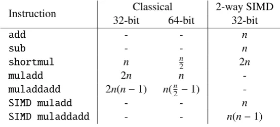
Table 1: A simplified comparison, only stating the number of word-level instructions required, to compute the Montgomery multiplication when using a 32n-bit modulus for a positive even integer
n. Two approaches are shown, a sequential one on the classical ALU (Algorithm 2 on page 5) and a parallel one using 2-way SIMD instructions (performing two operations in parallel, cf. Algorithm 4 on the previous page).
Instruction Classical 2-way SIMD 32-bit 64-bit 32-bit
add - - n
sub - - n
shortmul n n2 2n
muladd 2n n
-muladdadd 2n(n−1) n(n2 −1)
-SIMD muladd - - n
SIMD muladdadd - - n(n−1)
a simplified comparison based on the number of arithmetic operations when computing Montgomery multiplication using a 32n-bit modulus for a positive even integern. We denote bymuladdw(e,a,b,c) andmuladdaddw(e,a,b,c,d) the computation ofe = ab+c ande = ab+c+d, respectively, for 0 ≤ a,b,c,d < 2w (and thus 0 ≤ e < 22w). These are basic operations on a computer architecture which works onw-bit words. Some platforms have these operations as a single instruction (e.g., on some ARM architectures) while others implement this using separate multiplication and addition in-structions (as on the x86 platform). Furthermore, letshortmulw(e,a,b) denotee =abmod 2w: this w×w→w-bit multiplication only computes the least significantwbits of the result and is faster than computing a full double-word product on most modern computer platforms.
Table 1 summarizes the expected performance of Algorithm 2 on page 5 and Algorithm 4 on the preceding page in terms of arithmetic operations only. The shifting and masking operations are omitted for simplicity as well as the operations required to compute the final conditional subtraction or addition. When just taking themuladdandmuladdaddinstructions into account it becomes clear from Table 1 that the SIMD approach uses exactly half the number of instructions compared to the 32-bit classical implementation and almost twice as many operations compared to the classical 64-bit implementations. However, the SIMD approach requires more operations to compute the value ofq
every iteration and has various other overheads (e.g., inserting and extracting values from the large vector registers). Hence, when assuming that all the characteristics of the SIMD and classical (non-SIMD) instructions are identical, which is most likely not the case on most platforms, then we expect Algorithm 4 running on a 2-way 32-bit SIMD unit to outperform a classical 32-bit implementation using Algorithm 2 by at most a factor of two while being roughly half as fast as a classical 64-bit implementation.
4.2 A column-wise SIMD approach
on a lower level, while the approach from Section 4.1 above computes the arithmetic operations itself sequentially but divides the work into two steps which can be computed concurrently.
4.2.1 The Cell broadband engine
The Cell Broadband Engine (cf. the introductions given by Hofstee [41] and Gschwind [34]), denoted by “Cell” and jointly developed by Sony, Toshiba, and IBM, is a powerful heterogeneous multipro-cessor which was released in 2005. The Cell contains aPower Processing Element, a dual-threaded Power architecture-based 64-bit processor with access to a 128-bit AltiVec/VMX single instruction, multiple data (SIMD) unit (which is not considered in this chapter). Its main processing power, how-ever, comes from eightSynergistic Processing Elements (SPEs). For an introduction to the circuit design see the work by Takahashi et al. [73]. Each SPE consists of a Synergistic Processing Unit (SPU), 256 KB of private memory called Local Store (LS), and a Memory Flow Controller (MFC). To avoid the complexity of sending explicit direct memory access requests to the MFC, all code and data must fit within the LS.
Each SPU runs independently from the others at 3.192GHz and is equipped with a large register file containing 128 registers of 128 bits each. Most SPU instructions work on 128-bit operands de-noted asquadwords. The instruction set is partitioned into two sets: one set consists of (mainly) 4-and 8-way SIMD arithmetic instructions on 32-bit 4-and 16-bit oper4-ands respectively, while the other set consists of instructions operating on the whole quadword (including the load and store instructions) in a single instruction, single data (SISD) manner. The SPU is an asymmetric processor; each of these two sets of instructions is executed in a separate pipeline, denoted by theevenandoddpipeline for the SIMD and SISD instructions, respectively. For instance, the {4, 8}-way SIMD left-rotate instruction is an even instruction, while the instruction left-rotating the full quadword is dispatched into the odd pipeline. When dependencies are avoided, a single pair consisting of one odd and one even instruction can be dispatched every clock cycle.
One of the first applications of the Cell processor was to serve as the brain of Sony’s PlaySta-tion 3 game console. Due to the wide-spread availability of this game console and the fact that one could install and run one’s own software this platform has been used to accelerate cryptographic op-erations [27, 26, 23, 57, 18, 9] as well as cryptanalytic algorithms [69, 16, 14].
4.2.2 Montgomery multiplication on the Cell broadband engine
In this section we outline the approach presented by the first author of this chapter and Kaihara tailored towards the instruction set of the Cell Broadband Engine. Most notably, the presented techniques rely on an efficient 4-way SIMD instruction to multiply two 16-bit integers and add another 16-bit integer to the 32-bit result, and a large register file. Therefore, the approach described here uses a radix
r = 216 to divide the large numbers into words that match the input sizes of the 4-SIMD multipliers of the Cell. This can easily be adapted to any other radix size for different platforms with different SIMD instructions.
X =
Xs−1 =
128-bit length vector
z }| { 16-bit
|{z}
high
16-bit
|{z}
low
x3s−1 x2s−1 xs−1
... ...
Xj =
x3s+j x2s+j xs+j xj
... ...
X0 =
x3s x2s xs x0
| {z } the least significant 16-bit word ofX
Figure 1: The 16-bit words xi of a 16(n+1)-bit positive integer X = Pni=0xi216i < 2N are stored column-wise using s=ln+41m128-bit vectors Xjon the SPE architecture.
16-bit word is required because the intermediate accumulating result of Montgomery multiplication can be almost as large as 2N(see page 9 in Section 2.4).
The 16-bit digits xi are placed column-wisein the four 32-bit datatypes of the 128-bit vectors. This representation is illustrated in Figure 1. The four 32-bit parts of the j-th 128-bit vector Xj are denoted by
Xj ={Xj[3],Xj[2],Xj[1],Xj[0]}.
Each of the (n+ 1) 16-bit words xi of X is stored in the most significant 16 bits of Ximods[ ji
s k
]. The motivation for using this column-wise representation is that a division by 216 can be computed efficiently: simply move the digits in vectorX0“one position to the right”, which in practice means a logical 32-bit right shift, and relabeling of the indices such thatXjbecomesXj−1, for 1≤ j< s−1 and the modified vectorX0becomes the newXs−1. Algorithm 5 on the next page computes Montgomery multiplication using such a 4-way column-wise SIMD representation.
In each iteration, the indices of the vectors that contain the accumulating partial productUchange cyclically among thesregisters. In Algorithm 5, each 16-bit word of the inputs X,Y andN and the outputZ is stored in the upper part (the most significant 16 bits) of each of the four 32-bit words in a 128-bit vector. The vector µcontains the replicated values of−N−1mod 216 in the lower 16-bit positions of the four 32-bit words. In its most significant 16-bit positions, the temporary vectorK
stores the replicated values ofyi, i.e., each of the parsed coefficients of the multiplierYcorresponding to the i-th iteration of the main loop. The operation A ← muladd(B, c, D), which is a single instruction on the SPE, represents the operation of multiplying the vectorB(where data are stored in the higher 16-bit positions of 32 bit words) by a vector with replicated 16-bit values ofc across all higher positions of the 32-bit words. This product is added toD(in 4-way SIMD manner) and the overall result is placed intoA.
The temporary vectorVstores the replicated values ofu0in the least significant 16-bit words. This u0refers to the least significant 16-bit word of the updated value ofU, whereU = Pnj=0uj216j and is stored assvectors of 128-bit Uimods,Ui+1 mods, . . . ,Ui+nmods (whereirefers to the index of the main loop). The vectorQis computed as an element-wise logical left shift by 16 bits of the 4-SIMD product of vectorsV andµ.
Algorithm 5Montgomery multiplication algorithm for the Cell Input:
Nrepresented bys128-bit vectors: Ns−1, . . . ,N0, such that 216(n−1)≤N <216n, 2-N,
X,Yeach represented bys128-bit vectors:Xs−1, . . . ,X0, and Ys−1, . . . ,Y0, such that 0≤X,Y <2N,
µ: a 128-bit vector containing (−N)−1 (mod 216) replicated in all 4 elements.
Output:
(
Zrepresented bys128-bit vectors:Zs−1, . . . ,Z0, such that Z ≡XY2−16(n+1) modN, 0≤Z <2N.
1: for j=0 tos−1do
2: Uj=0
3: end for
4: fori=0 tondo
5: /* lines 6-9 computeU=yiX+U*/
6: K ={yi, yi, yi, yi}
7: for j=0 tos−1do
8: U(i+j) mods=muladd(Xj, K, U(i+j) mods)
9: end for
10: Carry propagation on U(i+j) modsfor j=0, . . . ,s−1(see text)
11: /* lines 12-13 computeQ=µV mod 216*/
12: V ={u0, u0, u0, u0}
13: Q=shiftleft(mul(V,µ), 16)
14: /* lines 15-17 computeU =NQ+U*/
15: for j=0 tos−1do
16: U(i+j) mods=muladd(Nj, Q, U(i+j) mods)
17: end for
18: Carry propagation on U(i+j) modsfor j=0, . . . ,s−1(see text)
19: /* line 20 computes the division by 216*/
20: Uimods=vshiftright(Uimods,32)
21: end for
22: Carry propagation on Uimodsfor i=n+1, . . . ,2n+1(see text)
23: for j=0 tos−1do
24: Zj=U(n+j+1) mods
25: end for
16-bit positions of temporary vectors. These vectors are then added to the “next” vectorU(i+j+1) mods correspondingly. The operation is carried out for the vectors with indices j ∈ {0,1, . . . ,s−2}. For
j = s−1, the last index, the temporary vector that contains the words is logically shifted 32 bits to the left and added to the vector Uimods. Similarly, the carry propagation of the higher words of U(i+j) mods in line 22 of Algorithm 5 is performed with 16-bit word extraction and addition, but requires a sequential parsing over the (n+1) 16-bit words.
Note, however, that an implementation of this technique outperforms the native multi-precision big-number library on the Cell processor by a factor of about 2.5, as summarized in [13].
4.3 Montgomery multiplication using the residue number system representation
The residue number system (RNS) as introduced by Garner [31] and Merrill [53] is an approach, based on the Chinese remainder theorem, to represent an integer as a number of residues modulo smaller (coprime) integers. The advantage of RNS is that additions, subtractions and multiplication can be performed independently and concurrently on these smaller residues. Given anRNS basisβn =
{r1,r2, . . . ,rn}, where gcd(ri,rj) = 1 fori, j, theRNS modulusis defined asR =Qni=1ri. Given an integer x∈Z/RZand the RNS basisβn, this integer xis represented as ann-tuple~x=(x1,x2, . . . ,xn) where xi = xmodri for 1 ≤ i≤ n. In order to convert ann-tuple back to its integer value one can apply the Chinese remainder theorem (CRT)
x= n X
i=1 xi R ri !−1 modri
R ri mod
R. (7)
Modular multiplication using Montgomery multiplication in the RNS setting has been studied, for instance, by Posch and Posch in [61] and by Bajard, Didier, and Kornerup in [4] and subsequent work. In this section we outline how to achieve this. First note for the application in which we are interested, we can not use the modulusNas the RNS modulus sinceNis either prime (in the setting of elliptic curve cryptography) or a product of two large primes (when using RSA). When computing the Montgomery reduction one has to perform arithmetic modulo the Montgomery radix. One possible approach is to use the RNS modulusR = Qni=1ri as the Montgomery radix. This has the advantage that whenever one computes with integers represented in this residue number system they are reduced moduloRimplicitly. However, since we are performing arithmetic in the ringZ/RZthis means that
division byR, as required in the Montgomery reduction, is not well-defined.
One way this problem can be circumvented is by introducing an auxiliary basisβ0n={r01,r02, . . . ,r0n} with auxiliary RNS modulusR0 =Qni=1r0i such that
gcd(R0,R)=gcd(R,N)=gcd(R0,N)=1
(and bothRandR0are larger than 4N). The idea is to convert the intermediate result represented inβn to the auxiliary basisβ0nand perform the division byRhere (sinceRandR
0
are coprime this inverse exists).
The concept of base-extension, converting the representation from one base to another, is by Szabo and Tanaka in [71] (but see also the work by Gregory and Matula in [33]). Methods are either based on the CRT as used by Shenoy and Kumaresan [67], Posch and Posch [60], and Kawamura, Koike, Sano, and Shimbo [46] or on an intermediate representation denoted by amixed radix systemas presented in Szabo and Tanaka in [71]. Carefully selected RNS bases can significantly impact the performance in practice as shown by Bajard, Kaihara, and Plantard in [3] and Bigou and Tisserand in [8]. Another RNS approach is presented by Phillips, Kong, and Lim [59].
With these two RNS bases defined we can compute the Montgomery product modulo N. Let
1. Compute the product ofAandBin both RNS basesβnandβ0n:
~
d=~a·~b, where di =aibi modri, for 1≤i≤n,
~
d0=a~0·b~0 where d0 i =a
0 ib
0 i modr
0
i for 1≤i≤n.
2. Compute ((ab)(−N−1modR) modR). This is realized by computingq~=−N~−1·d~in basisβnas qi =−Ni−1di modrifor 1≤i≤n.
3. Convert~qin basisβntoq~0in basisβ0n(for instance using Equation (7)).
4. Compute the final partc~0=(d~0+q~0·N~0)·R~−1of the Montgomery multiplication (including the division byR) in basisβ0nby computingc0i =(d
0 i +q
0 iN
0 i)r
−1 i modr
0
i for 1≤i≤n. 5. Convertc~0in basisβ0
nto~cin basisβn(for instance using Equation (7)).
After step 5 we have~c={c1,c2, . . . ,cn}andc~0={c01,c02, . . . ,c0n}such that
ci ≡
abR−1 modNmodri and c0i ≡
abR−1modNmodr0i.
This approach has been used to implement asymmetric cryptography on highly parallel computer ar-chitectures like graphics processing units (e.g., as in [5, 56, 72, 38, 2]). The results presented in these papers show that whenmultipleMontgomery multiplications are computed concurrently using RNS the latency can be reduced significantly while the throughput is increased (compared to computa-tion on a multi-core CPU) when computing with thousands of threads on the hundreds of cores on a graphics processing unit. This highlights the potential of using graphics cards as cryptographic accel-erators when large batches of work require processing (and a low latency is required). The process is illustrated in the example below.
LetA = 42,B = 17 and N = 67. In this example we show how to compute the Montgomery productABR−1 modNusing a residue number system. Let us first define the two coprime RNS bases
β3={3,7,13} with RNS modulus R=3·7·13=273,
β0
3={5,11,17} with RNS modulus R
0=5·11·17=935,
such that both RNS moduli are larger than 4N. Recall that Rplays the role of both the RNS modulus as well as of the Montgomery radix. First, we need to represent the inputsAandBin both RNS bases:A=42 is represented as
• ~a={42 mod 3,42 mod 7,42 mod 13}={0,0,3}in basisβ3, • a~0={42 mod 5,42 mod 11,42 mod 17}={2,9,8}in basisβ0
3,
andB=17 is represented as
• ~b={17 mod 3,17 mod 7,17 mod 13}={2,3,4}in basisβ3, • b~0={17 mod 5,17 mod 11,17 mod 17}={2,6,0}in basisβ0
3.
Furthermore, we need to represent the precomputed Montgomery constantµ= −N−1modR= −67−1mod 273=110 in basisβ3
~µ={110 mod 3,110 mod 7,110 mod 13}={2,5,6},
as well as the modulusNin basisβ03
~
N0 ={67 mod 5,67 mod 11,67 mod 17}={2,1,16}.
Compute the first step: the product of these two numbers in both bases. This can be done in parallel for all the individual moduli
• d~=~a·~b={0·2 mod 3,0·3 mod 7,3·4 mod 13}={0,0,12},
• d~0 =a~0·b~0 ={2·2 mod 5,9·6 mod 11,8·0 mod 17}={4,10,0}.
Next, compute~q=d~·~µin basisβ3
~q=d~·~µ={0·2 mod 3,0·5 mod 7,12·6 mod 13}={0,0,7}.
Change the representation ofq: convert~q={0,0,7}, which is represented in basisβ3, toq~0which is represented in basisβ03. This can be done by first converting~qback to its integer representation following Equation (7) on page 21
q= 0· 273 3 −1 mod 3 273 3 + 0· 273 7 −1 mod 7 273 7 + 7· 273 13 −1 mod 13 273 13 mod 273
= 0+0+7·5·21 mod 273=189.
Fromqobtainq~0 = {189 mod 5,189 mod 11,189 mod 17} = {4,2,2}. The final step computes the resultcin basisβ03asc~0 =(d~0+q~0·N~0)·R~−1:
~
c0 =({4,10,0}+{4,2,2} · {2,1,16})· {2,5,1}
={4,5,15}.
When converting this to the integer representation we obtain
c= 4· 935 5 −1 mod 5 935 5 + 5· 935 11 −1 mod 11 935 11+ 15· 935 17 −1 mod 17 935 17 mod 935
This is indeed correct since
c =ABR−1modN
=42·17·(3·7·13)−1mod 67
=49.
Acknowledgements
The authors want to thank Robert Granger, Arjen K. Lenstra, Paul Leyland, and Colin D. Walter for feedback and suggestions. Peter Montgomery’s authorship ishonoris causa; all errors and inconsis-tencies in this chapter are the sole responsibility of the first author.
References
[1] T. Acar and D. Shumow. Modular reduction without pre-computation for special moduli. Tech-nical report, Microsoft Research, 2010. (Cited on page 12.)
[2] S. Antão, J.-C. Bajard, and L. Sousa. RNS-based elliptic curve point multiplication for massive parallel architectures. The Computer Journal, 55(5):629–647, 2012. (Cited on page 22.)
[3] J. Bajard, M. E. Kaihara, and T. Plantard. Selected RNS bases for modular multiplication. In J. D. Bruguera, M. Cornea, D. D. Sarma, and J. Harrison, editors, 19th IEEE Symposium on Computer Arithmetic – ARITH 2009, pages 25–32. IEEE Computer Society, 2009. (Cited on page 21.)
[4] J.-C. Bajard, L.-S. Didier, and P. Kornerup. An RNS montgomery modular multiplication algo-rithm.IEEE Trans. Computers, 47(7):766–776, 1998. (Cited on page 21.)
[5] J.-C. Bajard and L. Imbert. A full RNS implementation of RSA. IEEE Transactions on Com-puters, 53(6):769–774, June 2004. (Cited on page 22.)
[6] P. Barrett. Implementing the Rivest Shamir and Adleman public key encryption algorithm on a standard digital signal processor. In A. M. Odlyzko, editor, Advances in Cryptology – CRYPTO’86, volume 263 ofLecture Notes in Computer Science, pages 311–323. Springer, Hei-delberg, Aug. 1987. (Cited on page 2.)
[7] D. J. Bernstein. Curve25519: New Diffie-Hellman speed records. In M. Yung, Y. Dodis, A. Ki-ayias, and T. Malkin, editors,PKC 2006: 9th International Conference on Theory and Practice of Public Key Cryptography, volume 3958 ofLecture Notes in Computer Science, pages 207– 228. Springer, Heidelberg, Apr. 2006. (Cited on page 11.)
[8] K. Bigou and A. Tisserand. Single base modular multiplication for efficient hardware RNS implementations of ECC. In T. Güneysu and H. Handschuh, editors,Cryptographic Hardware and Embedded Systems – CHES 2015, volume 9293 of Lecture Notes in Computer Science, pages 123–140. Springer, Heidelberg, Sept. 2015. (Cited on page 21.)
[10] J. W. Bos, C. Costello, H. Hisil, and K. Lauter. Fast cryptography in genus 2. In T. Johansson and P. Q. Nguyen, editors,Advances in Cryptology – EUROCRYPT 2013, volume 7881 ofLecture Notes in Computer Science, pages 194–210. Springer, Heidelberg, May 2013. (Cited on pages 11 and 12.)
[11] J. W. Bos, C. Costello, H. Hisil, and K. Lauter. High-performance scalar multiplication using 8-dimensional GLV/GLS decomposition. In G. Bertoni and J.-S. Coron, editors,Cryptographic Hardware and Embedded Systems – CHES 2013, volume 8086 ofLecture Notes in Computer Science, pages 331–348. Springer, Heidelberg, Aug. 2013. (Cited on page 12.)
[12] J. W. Bos, C. Costello, P. Longa, and M. Naehrig. Selecting elliptic curves for cryptography: an efficiency and security analysis. J. Cryptographic Engineering, 6(4):259–286, 2016. (Cited on page 12.)
[13] J. W. Bos and M. E. Kaihara. Montgomery multiplication on the Cell. In R. Wyrzykowski, J. Dongarra, K. Karczewski, and J. Wasniewski, editors,Parallel Processing and Applied Math-ematics – PPAM 2009, volume 6067 of Lecture Notes in Computer Science, pages 477–485. Springer, Heidelberg, 2010. (Cited on pages 17 and 21.)
[14] J. W. Bos, M. E. Kaihara, T. Kleinjung, A. K. Lenstra, and P. L. Montgomery. Solving a 112-bit prime elliptic curve discrete logarithm problem on game consoles using sloppy reduction.
International Journal of Applied Cryptography, 2(3):212–228, 2012. (Cited on page 18.)
[15] J. W. Bos, T. Kleinjung, A. K. Lenstra, and P. L. Montgomery. Efficient SIMD arithmetic modulo a Mersenne number. In E. Antelo, D. Hough, and P. Ienne, editors,IEEE Symposium on Computer Arithmetic – ARITH-20, pages 213–221. IEEE Computer Society, 2011. (Cited on page 11.)
[16] J. W. Bos, T. Kleinjung, R. Niederhagen, and P. Schwabe. ECC2K-130 on cell CPUs. In D. J. Bernstein and T. Lange, editors,AFRICACRYPT 10: 3rd International Conference on Cryptol-ogy in Africa, volume 6055 of Lecture Notes in Computer Science, pages 225–242. Springer, Heidelberg, May 2010. (Cited on page 18.)
[17] J. W. Bos, P. L. Montgomery, D. Shumow, and G. M. Zaverucha. Montgomery multiplication using vector instructions. In T. Lange, K. Lauter, and P. Lisonek, editors,SAC 2013: 20th Annual International Workshop on Selected Areas in Cryptography, volume 8282 of Lecture Notes in Computer Science, pages 471–489. Springer, Heidelberg, Aug. 2014. (Cited on pages 13, 14, 15, and 16.)
[18] J. W. Bos and D. Stefan. Performance analysis of the SHA-3 candidates on exotic multi-core architectures. In S. Mangard and F.-X. Standaert, editors,Cryptographic Hardware and Embed-ded Systems – CHES 2010, volume 6225 ofLecture Notes in Computer Science, pages 279–293. Springer, Heidelberg, Aug. 2010. (Cited on page 18.)
[19] A. Bosselaers, R. Govaerts, and J. Vandewalle. Comparison of three modular reduction func-tions. In D. R. Stinson, editor,Advances in Cryptology – CRYPTO’93, volume 773 ofLecture Notes in Computer Science, pages 175–186. Springer, Heidelberg, Aug. 1994. (Cited on page 2.)
[21] E. F. Brickell. A fast modular multiplication algorithm with application to two key cryptography. In D. Chaum, R. L. Rivest, and A. T. Sherman, editors,Advances in Cryptology – CRYPTO’82, pages 51–60. Plenum Press, New York, USA, 1982. (Cited on page 14.)
[22] Ç. K. Koç, T. Acar, and B. S. Kaliski Jr. Analyzing and comparing Montgomery multiplication algorithms. IEEE Micro, 16(3):26–33, 1996. (Cited on page 6.)
[23] H.-C. Chen, C.-M. Cheng, S.-H. Hung, and Z.-C. Lin. Integer number crunching on the Cell processor. International Conference on Parallel Processing, pages 508–515, 2010. (Cited on page 18.)
[24] J. Chung and M. A. Hasan. Montgomery reduction algorithm for modular multiplication us-ing low-weight polynomial form integers. In 18th IEEE Symposium on Computer Arithmetic (ARITH-18), pages 230–239. IEEE Computer Society, 2007. (Cited on page 12.)
[25] S. Cook. On the minimum computation time of functions. PhD thesis, Harvard University, 1966. (Cited on page 6.)
[26] N. Costigan and P. Schwabe. Fast elliptic-curve cryptography on the cell broadband engine. In B. Preneel, editor,AFRICACRYPT 09: 2nd International Conference on Cryptology in Africa, volume 5580 ofLecture Notes in Computer Science, pages 368–385. Springer, Heidelberg, June 2009. (Cited on page 18.)
[27] N. Costigan and M. Scott. Accelerating SSL using the vector processors in IBM’s cell broadband engine for sony’s playstation 3. Cryptology ePrint Archive, Report 2007/061, 2007. http:
//eprint.iacr.org/2007/061. (Cited on page 18.)
[28] B. Dixon and A. K. Lenstra. Massively parallel elliptic curve factoring. In R. A. Rueppel, editor,
Advances in Cryptology – EUROCRYPT’92, volume 658 ofLecture Notes in Computer Science, pages 183–193. Springer, Heidelberg, May 1993. (Cited on pages 12 and 14.)
[29] S. R. Dussé and B. S. Kaliski Jr. A cryptographic library for the Motorola DSP56000. In I. Damgård, editor,Advances in Cryptology – EUROCRYPT’90, volume 473 ofLecture Notes in Computer Science, pages 230–244. Springer, Heidelberg, May 1991. (Cited on pages 6, 7, and 8.)
[30] M. Fürer. Faster integer multiplication. In D. S. Johnson and U. Feige, editors,39th Annual ACM Symposium on Theory of Computing, pages 57–66. ACM Press, June 2007. (Cited on page 6.)
[31] H. L. Garner. The residue number system. InPapers Presented at the the March 3-5, 1959, West-ern Joint Computer Conference, IRE-AIEE-ACM ’59 (Western), pages 146–153, New York, NY, USA, 1959. ACM. (Cited on page 21.)
[32] R. Granger and A. Moss. Generalised Mersenne numbers revisited. Math. Comput., 82(284):2389–2420, 2013. (Cited on page 12.)
[34] M. Gschwind. The Cell broadband engine: Exploiting multiple levels of parallelism in a chip multiprocessor. International Journal of Parallel Programming, 35:233–262, 2007. (Cited on page 18.)
[35] S. Gueron and V. Krasnov. Fast prime field elliptic-curve cryptography with 256-bit primes. J. Cryptographic Engineering, 5(2):141–151, 2015. (Cited on page 13.)
[36] G. Hachez and J.-J. Quisquater. Montgomery exponentiation with no final subtractions: Im-proved results. In Ç. K. Koç and C. Paar, editors, Cryptographic Hardware and Embedded Systems – CHES 2000, volume 1965 of Lecture Notes in Computer Science, pages 293–301. Springer, Heidelberg, Aug. 2000. (Cited on page 9.)
[37] M. Hamburg. Fast and compact elliptic-curve cryptography. Cryptology ePrint Archive, Report 2012/309, 2012. http://eprint.iacr.org/2012/309. (Cited on page 12.)
[38] O. Harrison and J. Waldron. Efficient acceleration of asymmetric cryptography on graphics hardware. In B. Preneel, editor,AFRICACRYPT 09: 2nd International Conference on Cryptol-ogy in Africa, volume 5580 of Lecture Notes in Computer Science, pages 350–367. Springer, Heidelberg, June 2009. (Cited on page 22.)
[39] L. Hars. Long modular multiplication for cryptographic applications. In M. Joye and J.-J. Quisquater, editors, Cryptographic Hardware and Embedded Systems – CHES 2004, volume 3156 of Lecture Notes in Computer Science, pages 45–61. Springer, Heidelberg, Aug. 2004. (Cited on page 12.)
[40] K. Hensel.Theorie der algebraischen Zahlen. Tuebner, Leipzig, 1908. (Cited on page 2.)
[41] H. P. Hofstee. Power efficient processor architecture and the Cell processor. In High-Performance Computer Architecture – HPCA 2005, pages 258–262. IEEE, 2005. (Cited on page 18.)
[42] K. Iwamura, T. Matsumoto, and H. Imai. Systolic-arrays for modular exponentiation using Montgomery method (extended abstract) (rump session). In R. A. Rueppel, editor, Advances in Cryptology – EUROCRYPT’92, volume 658 of Lecture Notes in Computer Science, pages 477–481. Springer, Heidelberg, May 1993. (Cited on page 14.)
[43] M. E. Kaihara and N. Takagi. Bipartite modular multiplication. In J. R. Rao and B. Sunar, editors,Cryptographic Hardware and Embedded Systems – CHES 2005, volume 3659 ofLecture Notes in Computer Science, pages 201–210. Springer, Heidelberg, Aug./Sept. 2005. (Cited on page 14.)
[44] A. A. Karatsuba and Y. Ofman. Multiplication of many-digital numbers by automatic computers.
Doklady Akad. Nauk SSSR, 145(2):293–294, 1962. Translation in Physics-Doklady7, pp. 595– 596, 1963. (Cited on page 6.)
[45] E. Käsper. Fast elliptic curve cryptography in OpenSSL. In G. Danezis, S. Dietrich, and K. Sako, editors,FC 2011 Workshops, volume 7126 ofLecture Notes in Computer Science, pages 27–39. Springer, Heidelberg, Feb./Mar. 2012. (Cited on page 11.)
volume 1807 ofLecture Notes in Computer Science, pages 523–538. Springer, Heidelberg, May 2000. (Cited on page 21.)
[47] M. Kneževi´c, F. Vercauteren, and I. Verbauwhede. Speeding up bipartite modular multiplication. In M. A. Hasan and T. Helleseth, editors,Arithmetic of Finite Fields – WAIFI, volume 6087 of
Lecture Notes in Computer Science, pages 166–179. Springer, 2010. (Cited on page 12.)
[48] D. E. Knuth.Seminumerical Algorithms. The Art of Computer Programming. Addison-Wesley, Reading, Massachusetts, USA, 3rd edition, 1997. (Cited on page 2.)
[49] N. Koblitz. Elliptic curve cryptosystems.Mathematics of Computation, 48(177):203–209, 1987. (Cited on page 11.)
[50] Çetin Kaya. Koç and T. Acar. Montgomery multiplication in GF(2k). Designs, Codes and Cryptography, 14(1):57–69, 1998. (Cited on page 10.)
[51] P. C. Kocher, J. Jaffe, and B. Jun. Differential power analysis. In M. J. Wiener, editor,Advances in Cryptology – CRYPTO’99, volume 1666 ofLecture Notes in Computer Science, pages 388– 397. Springer, Heidelberg, Aug. 1999. (Cited on pages 2 and 8.)
[52] A. K. Lenstra. Generating RSA moduli with a predetermined portion. In K. Ohta and D. Pei, editors,Advances in Cryptology – ASIACRYPT’98, volume 1514 ofLecture Notes in Computer Science, pages 1–10. Springer, Heidelberg, Oct. 1998. (Cited on page 12.)
[53] R. D. Merrill. Improving digital computer performance using residue number theory.Electronic Computers, IEEE Transactions on, EC-13(2):93–101, April 1964. (Cited on page 21.)
[54] V. S. Miller. Use of elliptic curves in cryptography. In H. C. Williams, editor, Advances in Cryptology – CRYPTO’85, volume 218 ofLecture Notes in Computer Science, pages 417–426. Springer, Heidelberg, Aug. 1986. (Cited on page 11.)
[55] P. L. Montgomery. Modular multiplication without trial division.Mathematics of Computation, 44(170):519–521, April 1985. (Cited on pages 1, 4, 6, and 7.)
[56] A. Moss, D. Page, and N. P. Smart. Toward acceleration of RSA using 3D graphics hardware. In S. D. Galbraith, editor, 11th IMA International Conference on Cryptography and Coding, volume 4887 ofLecture Notes in Computer Science, pages 364–383. Springer, Heidelberg, Dec. 2007. (Cited on page 22.)
[57] D. A. Osvik, J. W. Bos, D. Stefan, and D. Canright. Fast software AES encryption. In S. Hong and T. Iwata, editors, Fast Software Encryption – FSE 2010, volume 6147 ofLecture Notes in Computer Science, pages 75–93. Springer, Heidelberg, Feb. 2010. (Cited on page 18.)
[58] D. Page and N. P. Smart. Parallel cryptographic arithmetic using a redundant Montgomery representation. IEEE Trans. Computers, 53(11):1474–1482, 2004. (Cited on page 14.)
[59] B. J. Phillips, Y. Kong, and Z. Lim. Highly parallel modular multiplication in the residue number system using sum of residues reduction.Appl. Algebra Eng. Commun. Comput., 21(3):249–255, 2010. (Cited on page 21.)
[60] K. Posch and R. Posch. Base extension using a convolution sum in residue number systems.