A simulation study of effects of GRACE orbit decay on the gravity field
recovery
Keiko Yamamoto1, Toshimichi Otsubo2, Toshihiro Kubo-oka2, and Yoichi Fukuda1
1Department of Geophysics, Graduate School of Science, Kyoto University, Kitashirakawa Oiwake-cho, Sakyo-ku, Kyoto 606-8502, Japan 2National Institute of Information and Communications Technology, 893-1, Hirai, Kashima, Ibaraki 314-8501, Japan
(Received November 22, 2004; Revised February 19, 2005; Accepted February 19, 2005)
The effects of satellite ground track changes of GRACE on monthly gravity field recoveries are investigated. In the case of a gravity field recovery using a relatively short period of a month or so, the variation of ground tracks affects the precision of the gravity field solutions. It is a serious problem when the solutions are employed for detecting temporal gravity changes which are almost at their detection limits. In this study, the recoveries of four-weekly gravity fields are simulated and the relation between the recovery precision and the ground track is investigated. The result shows that the GRACE ground track of the year 2003 was in good condition for four-week gravity field recovery, but it will sometimes appear as worse cases as the orbit altitude decays. In those cases, the global standard deviations of geoid height errors will be about one order worse than the best case. From our simulation, ground tracks of around altitudes of 473, 448, 399, 350 and 337 km give insufficient spatial resolutions, even for gravity field recovery up to degree 30.
Key words:Satellite gravity mission, GRACE, gravity field, satellite orbit.
1.
Introduction
The dedicated gravity mission GRACE (Gravity Recov-ery and Climate Experiment, Tapleyet al., 2004) provides monthly gravity-field solutions throughout the mission’s lifetime for the purpose of detecting temporally varying geophysical phenomena. To detect these signals precisely, we should characterize the errors which degrade the quality of the gravity-field solutions. The aliasing effects causing short-term mass variations in the atmosphere or the ocean, are one of the most serious errors in the gravity-field re-covery from satellite data. Hanet al.(2004) estimated the aliasing effects on the monthly mean GRACE gravity solu-tions due to the mismodeling of ocean tides and atmosphere and due to ground-surface water mass variation. The result shows that these errors corrupt recovered coefficients and introduce large errors in global monthly geoid solutions. In fact, the errors still remain in the monthly solutions though de-aliasing atmospheric and oceanic models are used in the real GRACE data processing.
Apart from these effects, the ground track variations caused by the orbit decay also affect the precision of the recovery of the gravity field. During the mission’s lifetime, the GRACE satellite is not maintained to keep the same or-bit due to thruster fuel limitations (Caseet al., 2004). The orbit decays from an initial altitude of about 500 km to an end-of-mission altitude of 300 km. This causes temporal variation of the ground track of the satellite. For the gravity field solutions, globally uniform ground tracks is preferred, but large gaps in the ground tracks appear at a specific
or-Copy right cThe Society of Geomagnetism and Earth, Planetary and Space Sci-ences (SGEPSS); The Seismological Society of Japan; The Volcanological Society of Japan; The Geodetic Society of Japan; The Japanese Society for Planetary Sci-ences; TERRAPUB.
bit altitude. Large gaps are compensated by using relatively long period data. Therefore, in the case of CHAMP (CHAl-lenging Minisatellite Payload, Reigberet al., 2002) it does not effect the mission which recovers the static gravity field using some months or years of data. However, in the case of a gravity field recovery such as the GRACE mission, a relatively short period data of a month or so are used and the variation of ground tracks affects the precision of the gravity-field solutions. It presents a serious problem when the solutions are used for the detection of temporal gravity changes which are around the detection limits.
Although the main purpose of the CHAMP mission is the detection of a static gravity field, Sneeuwet al.(2003) attempted to detect time-varying signals from monthly CHAMP solutions. They proved that the error level was too large to detect time-varying signals and stated that the ground track variation of the CHAMP satellite is one of the main contributors.
In this paper, with the GRACE data in mind, the monthly gravity field recovery data from a temporally decaying orbit satellite is simulated and the impact of the satellite’s ground track to the precision of the recovery of the gravity field is quantified.
2.
Simulation Procedure
The outline of our simulation procedure is as follows. Firstly, the simulated orbit of the GRACE satellite was gen-erated. Secondly, the geopotential value along the orbit was calculated from the known spherical harmonic coef-ficients. A stochastic error model was introduced and the ‘observational’ value was synthesized by adding the error to the geopotential value. Thirdly, spherical harmonic coef-ficients were recovered from four-week observational data
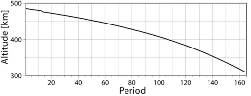
Fig. 1. Temporal decay of the simulated mean orbit altitude. The simulated orbit was divided into periods of 4 weeks (more details are shown in Subsection 2.1), and the period numbers of 4 weeks are shown at the x-axis of the graph.
Fig. 2. Global standard deviations of the geoid height error calculated from the difference of recovered and true (original) spherical harmonic coefficients at each time period. The simulated orbit was divided to periods of 4 weeks (more details are shown in Subsection 2.1), and the period numbers of 4 weeks are shown at the x-axis of the graph.
using the least-squares method (LSM). Finally, recovered coefficients were compared to the original ones and the pre-cision of the recovery of the gravity field was estimated. Details of each procedure are stated in the following sub-sections.
2.1 Preparation of the simulated GRACE orbit
In view of the requirements of the GRACE mission, a satellite orbit above an altitude of 300 km was prepared for our simulation. Satellite orbits for the first year were pre-pared from all two-line element (TLE) sets of GRACE-1 of the year 2003. The time interval of each TLE set was 1 day or less. The orbits after that were numerically inte-grated from the last GRACE-1 TLE set of the year 2003. The orbit was generated by an SGP4 model (Hoots and Roehrich, 1980). Satellite positions per 10 sec were calcu-lated. Figure 1 shows the time variation of the mean altitude (mean semimajor axis minus the mean equatorial radius of the Earth) of the simulated orbit. Orbit data was divided into 4 weeks and the gravity field recovery was simulated using the data sets of each time period.
2.2 Simulation of gravity-field observations from satel-lite positions
To improve the signal attenuation to a high degree, range-rate measurement using two satellites was adopted in the real GRACE mission. However, as our interest is the error from ground track variation and not the one from the higher-degree signal attenuation, a two-satellite approach is not necessary. Therefore, in order to simplify our simulation, we assumed that the geopotential was observed from one satellite.
The Earth’s real gravity field is temporally changing
be-cause of the time-variation of the mass distribution of the atmosphere, ocean, land water, and so on. However, in our simulation, a static gravity field was assumed to eliminate the aliasing effects of such temporally varying signals and to see only the error from ground-track variations.
In this study, the GGM01C model (Center for Space Re-search, 2003) was assumed as the Earth’s ‘true’ geopoten-tial model. ‘Observational’ data of the gravity field was generated by calculating the geopotential value from each satellite position and the ‘true’ gravity field coefficients by
Vobs(φ, λ,r)=
G M R
L
l=2 R r
l+1l
m=0
¯
Plm(sinφ)
×(C¯ln(tr ue)cosmλ+ ¯Slm(tr ue)sinmλ)
+εV, (1)
whereVobsis the ‘observed’ geopotential,Gis the
gravita-tional constant, andM is the mass of the Earth. φ,λandr
are the geocentric latitude, longitude and radius of the ob-servational point, respectively. Ris the Earth’s mean equa-tor radius.Lis the cut-off degree,P¯lm is a fully normalized
associated Legendre function, andC¯lm(tr ue)andS¯lm(tr ue)are
fully normalized ‘true’ spherical harmonic coefficients. εV
is the observational error. The cut-off degreeL was set to 30 for this study.
2.3 Introduction of observational error
A geopotential error equivalent to the inter-satellite range-rate measurement error of Low-Low Satellite-to-Satellite Tracking (LL-SST) was calculated and substituted for the observational error εV in Eq. (1). We assumed
that for GRACE (<1μm/s) (Goddard Space Flight Center, 2002). We assumed an energy balance approach to derive the geopotential value from the observational data of the GRACE satellite (range rate). The velocity error was con-verted to the corresponding geopotential error by utilizing the law of energy conservation (Rapp and Jekeli, 1981):
εV =εvelocity
G M
r , (2)
whereεvelocityis the range-rate measurement error andεV is
the corresponding geopotential error. The geopotential er-ror was estimated for each altitude. A Gauss-distributed random error was assumed and added to the observed geopotential as shown in Eq. (1). A 1μm/s range-rate mea-surement error corresponds to a 0.0076 m2/s2 error of the geopotential and a 0.78 mm error of the geoid height when the orbit altitude (rminus the mean equatorial radius of the Earth) is assumed to be 450 km.
2.4 Recovery of gravity field and estimation of recov-ery precision
Using the linear LSM, the gravity field at each time pe-riod was recovered from the corresponding four-week set of every 10-sec observational equations. The estimated pa-rameters were fully normalized spherical harmonic coeffi-cients,C¯lm(calc)andS¯lm(calc)up to degree/order 30. A
space-wise approach was adopted in our simulation.
Because of the near-polar orbit of the satellite, the distri-bution of the observation points becomes heterogeneous in the latitudinal direction, that is, the distribution of the obser-vation points is dense near the poles and sparse around the equator. Therefore, the recovery error of the gravity field becomes small near the poles and large around the equator. In our simulation, the difference in the recovery precision caused by ground-track variation is estimated using a global standard deviation (see Section 3). To see only the effect of ground-track variation clearly, we exclude the above effect by using the proper weight in the LSM. The weight was set so that it would cancel the heterogeneous distribution of the observational points in the latitudinal direction. The weight at the observational point j is
wj=
1
nj,
(3)
wherenj is the number of points per unit area at j.
The recovery precision of each four-week period was evaluated by comparing the calculated spherical harmonic coefficients with the ‘true’ (original) ones.
3.
Comparison of Satellite Ground Track with
Gravity Field Recovery
Geoid height errors were calculated from the difference between the recovered and true spherical harmonic coeffi-cients and the global standard deviations were calculated at each time period. Figure 2 shows the results. The re-covery errors shown in Fig. 2 are larger than those of the real GRACE mission (CSR, 2004). It comes from the dif-ference between the recovery methods. That is, (absolute) spherical harmonic coefficients were recovered in our sim-ulation, while monthly gravity-field solutions are estimated
from observational data by updating an a-priori best-known geopotential model in the real GRACE processing (Bettad-pur, 2003). Therefore, the error value in our simulation be-came larger from the effect of a computational round-off error. However, since our purpose here is to find the dif-ference in the recovery precision for each time period, this difference does not become a problem. In Fig. 2, global standard deviations were around 65 mm in most periods, but above 100 mm standard deviations can be seen in some periods.
In order to discuss the relation between the satellite ground track and recovery precision of the gravity field, spatial distribution of observational point at each period was transformed to spherical harmonic coefficients. Al-though the recovery of the gravity field was up to 30 de-grees, the cut-off degree of this spherical harmonic transfor-mation was set to 180 degrees so that the spectrum express a sufficiently small periodic pattern of ground track. From the derived spherical harmonic coefficients, the amplitude of degreeland orderm,
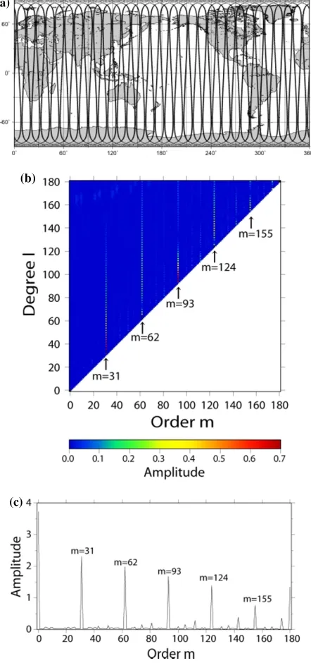
was calculated for eachlandm. As an example, the original observational point distribution (Fig. 3(a)) and the derived amplitude of eachl andm (Fig. 3(b)) of the period 108 are shown. Large amplitude coefficients are concentrated at several specific orders of m. To see the feature of the order of direction more clearly, an order amplitude was introduced as follows and calculated at each period:
σm=
whereσmis the order amplitude for each ordermandL is
the cut-off degree, that is, 180 in our simulation. Figure 3(c) shows the order amplitude spectrum of the period 108. Gen-erally, the large peak of ordermin Fig. 3(c) represents the fact that sampling points concentrate at the specific cycle which divide equator with 2mnodes. However, ifmis not a prime number, then the cycle does not necessarily divide the Equator with 2mnodes. The 2mnodal cycles perntimes (nis an integer number) revolution of the Earth also appear at the spectrum in the order ofm. For example, comparing Fig. 3(a) with (b) and (c), we see that the peak of order 62 in Fig. 3(b) and (c) has 2×62 nodal cycles per two revo-lutions, which corresponds to 2×31 nodal cycles per one revolution. Further, the residual large peaks at orders 93, 124 and 155 are also the multiple of the order 31, the 2×31 nodal cycles. Therefore the cycles of orders 31, 62, 93, 124 and 155 are superposed. These explanations are shown by the following formula:
°
(a)
(b)
(c)
Fig. 3. (a) Spatial distributions of observational points of period 108. (b) Amplitude of the eachlandm(Eq. (5)) derived from fully normalized spherical harmonic transformation of (a). (c) Order amplitude spectrum (Eq. (6)) derived from fully normalized spherical harmonic transformation of (a).
kis equal toβ in the exact orbit resonance conditionβ/α (whereαandβare co-prime integers and which represents
β revolutions, while the Earth rotatesαtimes) (Klokoˇcn´ık
et al., 2003). Therefore, n should be decided based on the information of the exact orbit resonance near the time period. In our approach, the amplitudes of the resonance components are estimated. Therefore, we can know how long the effect of this resonance continues though we cannot know the exact resonance point.
On the basis of (6), we estimated the actual ground-track separation N and corresponding order ofk for all original orders m of the containing cycles of each period. Power spectra of the same orderkwere added to each other. Each order (k) peak is maintained throughout some time periods. The orders (k) whose largest amplitudes (square root of power spectrum) are above 1.0 (except order (k) 0 and 180) are listed in Fig. 4.
The ground tracks of periods 1 to 13 corresponds to the real ground tracks of the GRACE-1 satellite. There are large peaks of order 137 in periods 2 to 8. However, the ground track separation of 137 is small enough to determine the gravity field up to degree/order 30. Therefore, the GRACE ground track of the year 2003 is a good condition for recov-ering the Earth’s gravity field, as shown in Fig. 2.
To confirm that our results are agreeable, the errors of 10 sets of GRACE monthly gravity field solutions up to de-gree/order 120 of the year 2003, released by the Center for Space Research (2004), were investigated. In the real pro-cessing of the GRACE observational data, the gravity-field solutions are estimated in a different way from our simula-tion (Bettadpur, 2003), but the quality of the derived gravity field is also affected by the distribution of the observational points. The ground-track separation of the cycle of order 137 is also sufficient to recover the gravity field up to de-gree/order 120. The error amplitudes per degree were com-puted from the coefficients’ formal (uncalibrated) standard deviations (data not shown). The result shows that the er-rors are about 40 mm at maximum and 20 mm at minimum, at degree 120, which are almost at the same level and an extremely large difference cannot be found. It shows that our simulation is agreeable.
However, after the end of 2003, large specific cycle peaks which gave large ground track separations appeared as the orbit decayed (Fig. 4). Some ground-track separations are too large to precisely determine the gravity field up to de-gree/order 30, as shown in Fig. 2. Such peaks correspond to the short-period repeating orbital cycles. For example, the large peak of the period 108 corresponds to the repeating cycles of 31 cycles per 2 sidereal days. Although such a specific cycle observation is useful to check or calibrate the corresponding specific degree/order of the derived spherical harmonic solutions (Klokoˇcn´ıket al., 2003), it is disadvan-tageous for global gravity field recovery.
4.
Discussion
The decay rate of the altitude in the real GRACE mis-sion may not be the same in our simulation. Therefore,
the length of period which gives large ground-track sepa-ration may also be different in our simulation, but such a period will appear because the order of cycles contained in each period are determined mainly by the orbital alti-tude. From our simulation, ground tracks of around period 19, 56, 107, 142 and 156, which correspond to the altitude (mean semimajor axis minus the mean equatorial radius of the Earth) 473, 448, 399, 350, and 337 km, respectively, give insufficient spatial resolutions for the gravity-field re-covery up to degree/order 30. When these solutions are used for detecting temporally changing geophysical phenomena, especially the phenomena near the detection limit, the pre-cise estimation of the signal cannot be expected because the information used for updating at such periods does not have a sufficiently high quality. For example, although the GRACE satellite has a sensitivity to detect seasonal changes of land water of 500 km half wavelength (National Research Council, 1997), the resolution is not sufficient if the large ground-track separation period lasts for a few months.
From the real GRACE orbital data, released with a monthly gravity field solution, we can estimate more ac-curately for how long such an insufficient resolution pe-riod continues. It is very important to know the quality of GRACE monthly gravity field solution.
References
Bettadpur, S.,Level-2 Gravity Field Product User Handbook, GRACE 327-734, CSR, 2003.
Case, K., G. Kruizinga, and S. C. Wu,GRACE Level 1B Data Product User Handbook, JPL D-22027, NASA, 2004.
Center for Space Research, GGM01 Notes, http://www.csr.utexas.edu/ grace/, 2003.
Center for Space Research, GRACE Level 2 products, http://podaac.jpl. nasa.gov/grace/, 2004.
Goddard Space Flight Center,GRACE Gravity Recovery and Climate Ex-periment, NP-2002-2-427-GSFC, NASA, 2002.
Han, S. C., C. Jekeli, and C. K. Shum, Time-variable aliasing effects of ocean tides, atmosphere, and continental water mass on monthly mean GRACE gravity field,J. Geophys. Res.,109, B04403, 2004.
Hoots, F. R. and R. L. Roehrich,Spacetrack Report No. 3 - Models for Propagation of NORAD Element Sets, 10 pp., Aerospace Defence Cen-ter, Peterson AFB, 1980.
Klokoˇcn´ık, J., J. Kosteleck´y, and R. H. Gooding, On fine orbit selection for particular geodetic and oceanographic missions involving passage through resonances,J. Geod.,77, 30–40, 2003.
National Research Council, SATELLITE GRAVITY AND THE GEO-SPHERE - Contributions to the study of the Solid Earth and Its Fluid Envelope, National Academy Press, Washington, D.C., 1997. Rapp, R. H. and C. Jekeli, Accuracy of the Determination of Mean
Anoma-lies and Mean Geoid Undulations from a Satellite Gravity Field Map-ping Mission, Rep. 307, Dept. of Geod. Sci. and Surv., Ohio State Univ., Columbus, 1981.
Reigber, C., H. L¨uhr, and P. Schwintzer, CHAMP mission status,Adv. Space Res.,30, 129–134, 2002.
Sneeuw, N., C. Gerlach, L. F¨oldv´ary, T. Gruber, T. Peters, R. Rummel, and D. ˇSvehla, One year of time-variable CHAMP-only gravity field models using kinematic orbits, inA Window on the Future of Geodesy, IAG Symposium 128, edited by F. Sanso, 288 pp., Springer, 2003. Tapley, B. D., S. Bettadpur, M. Watkins, and C. Reigber, The Gravity
Recovery and Climate Experiment: Mission overview and early results, Geophys. Res. Lett.,31, L09607, 2004.