Comparison of GPS receiver DCB estimation methods using a GPS network
Byung-Kyu Choi1, Jong-Uk Park1, Kyoung Min Roh1, and Sang-Jeong Lee2
1Space Science Division, Korea Astronomy and Space Science Institute, Daejeon 305-348, South Korea 2Department of Electronics Engineering, Chungnam National University, Daejeon 305-764, South Korea
(Received June 6, 2012; Revised October 10, 2012; Accepted October 10, 2012; Online published August 23, 2013)
Two approaches for receiver differential code biases (DCB) estimation using the GPS data obtained from the Korean GPS network (KGN) in South Korea are suggested: the relative and single (absolute) methods. The relative method uses a GPS network, while the single method determines DCBs from a single station only. Their performance was assessed by comparing the receiver DCB values obtained from the relative method with those estimated by the single method. The daily averaged receiver DCBs obtained from the two different approaches showed good agreement for 7 days. The root mean square (RMS) value of those differences is 0.83 nanoseconds (ns). The standard deviation of the receiver DCBs estimated by the relative method was smaller than that of the single method. From these results, it is clear that the relative method can obtain more stable receiver DCBs compared with the single method over a short-term period. Additionally, the comparison between the receiver DCBs obtained by the Korea Astronomy and Space Science Institute (KASI) and those of the IGS Global Ionosphere Maps (GIM) showed a good agreement at 0.3 ns. As the accuracy of DCB values significantly affects the accuracy of ionospheric total electron content (TEC), more studies are needed to ensure the reliability and stability of the estimated receiver DCBs.
Key words:Differential code biases, receiver, total electron content, GPS network.
1.
Introduction
The total electron content (TEC) in the ionosphere can be easily estimated from the combination of the Global Po-sitioning System (GPS) data. However, the TEC data de-rived from GPS measurements have an uncertainty because each GPS signal has a hardware-associated bias that seri-ously affects the accuracy of the ionospheric TEC estimates (Cocoet al., 1991; Lanyi and Roth, 1988). Hardware bi-ases in GPS signals are caused by GPS satellite transmitters and receivers (Sardonet al., 1994; Davies and Hartmann, 1997).
In general, GPS TEC is calculated with the so-called geometry-free linear combination of two frequencies (L1– L2). Hardware biases are usually determined in a relative aspect because they remain in the ionospheric TEC after subtracting measurements at different frequencies. These differences in the hardware biases of GPS code measure-ments are called differential code biases (DCBs) (Mannucci
et al., 1998; Meza, 1999). Choiet al. (2011) showed that
the receiver DCBs estimated from GPS measurements reach up to a few tens of nanoseconds. GPS satellite DCBs have a range at the level of a few nanoseconds (ns) and exhibit very gradual drifts over periods of several months. They have a long-term stability with a root mean square (RMS) error of about 0.2 ns (Wilson and Mannucci, 1994). These DCBs can seriously affect ionospheric TEC estimation. There-fore, it is necessary to precisely estimate GPS satellite and
Copyright cThe Society of Geomagnetism and Earth, Planetary and Space Sci-ences (SGEPSS); The Seismological Society of Japan; The Volcanological Society of Japan; The Geodetic Society of Japan; The Japanese Society for Planetary Sci-ences; TERRAPUB.
doi:10.5047/eps.2012.10.003
receiver DCBs to improve the accuracy of TEC estimates. Many studies have been introduced to separate DCBs from TEC. DCBs can be calculated from the data of GPS networks or a single station. Ma and Maruyama (2003) presented a method to estimate GPS satellite and receiver DCBs using the GPS Earth Observation Network (GEONET) in Japan. Maet al.(2005) also presented an ap-proach for single receiver DCB estimation using the Global Ionosphere Maps (GIMs) of the International GNSS Ser-vice (IGS). In this case, only receiver DCBs were esti-mated. However, the DCB values for all GPS satellites are presumably known from IGS GIM or other GIMs. The DCBs of the IGS GIMs are a combined solution from the following analysis centers (ACs): the Centre for Or-bit Determination in Europe (CODE) in Switzerland, the Jet Propulsion Laboratory (JPL) in the USA, the European Space Agency (ESA) in Germany, and the Technical Uni-versity of Catalonia (UPC) in Spain. The ACs deliver global maps in grid form of vertical total electron contents (VTEC) and DCB values in a common exchange format named the IONospheric EXchange (IONEX) by using GPS data from over 100 IGS stations with different methods (Schaeret al., 1998). GIMs have a spatial resolution of and in latitude and longitude, and a 2-hour temporal resolution (Feltens and Jakowski, 2002). DCB values for all GPS satellites and IGS stations are estimated as constant values for each day.
The influence of geomagnetic storms on the estimation of receiver DCBs in the China region was recently investi-gated by Zhanget al. (2009). Zhanget al. (2010) also car-ried out an accuracy analysis of GPS DCBs estimated from measurements in middle and low latitudes. The GPS re-ceiver DCBs are different depending on the type of rere-ceiver
and the temperature of the hardware (Gao and Liu, 2002). Hernandez-Pajareset al. (2009) showed receiver DCB val-ues ranging from−20 to+15 ns with a variability up to a few nanoseconds.
In this study, two approaches for receiver DCB estima-tion are suggested. One is to determine the receiver DCBs using a regional GPS network. However, one of the receiver DCBs needs to be set to an arbitrary reference value in or-der to avoid singularities in the parameter estimation pro-cess. Another approach is to calculate the DCBs from a single receiver only. We compare directly the results esti-mated by the two methods, and we consider their statistical values and stability.
2.
GPS DCB Estimation Approaches
GPS satellites transmit two signals on L-band frequen-cies L1 (1575.42 MHz) and L2 (1227.60 MHz). Dual-frequency GPS measurements are not only used to elimi-nate mostly the effect of the ionosphere, but also to estimate TEC in the ionosphere.
Methods for ionospheric TEC estimation have been de-scribed by many studies (Lanyi and Roth, 1988; Davies and Harmann, 1997; Sardon and Zarraoa, 1997; Hernandez-Pajareset al., 1999; Mannucciet al., 1999; Otsukaet al., 2002). We adopted the common model in which the iono-sphere consists of a thin shell at a fixed height, usually 350 km. The GPS receiver measures the slant TEC for each satellite.
When the GPS signals pass through the ionosphere, the TEC in the ionosphere imposes a dispersive delay on the navigation signals. This delay can be easily calculated from Eq. (1): is the frequency of the GPS signal. To obtain a better accu-racy for the GPS-TEC, carrier phase smoothing is employed with the code and carrier phase measurements.
We consider the slant TEC, STECi,j,k, measured along a
ray path between satellite-iand receiver-jat a time epochk
fori =1,2, . . . ,s, j =1,2, . . . ,r,k=1,2, . . . ,t, where
s is the number of the available satellite,r is the number of the receiver, andt is the number of the time series data. Assuming that the vertical TEC is a function of the satellite, the receiver, and the epoch, the vertical TEC is written as VTECi,j,k. The relationship between STECi,j,k, VTECi,j,k,
and the DCBs is as follows:
M·VTECi,j,k+bj+bi =STECi,j,k, (2)
wherebj andbi are C1-P2 DCB of the receiver and
satel-lite respectively. In Eq. (2), VTECi,j,k, bj and bi are
unknowns, the number of unknowns, which is equal to
s×r×t+s+r, exceeds the number of equations, which is equal to the number of the slant TECs(s×r×t). In this case, the equation cannot be solved. To solve this equation, we assume that the vertical TEC is invariant with the satel-lite and receiver. Consequently, the unknowns (VTECk, bj and bi) are obtained from equations whose number is
(s+r+t). The satellite and receiver DCBs are computed hourly as constant values using daily data. In our approach, the satellite DCB values are realigned to make the results comparable to the IGS results, which are based on a zero-mean condition, i.e. the sum of all satellite DCBs is forced to be zero. M is the ionospheric mapping function depen-dent on the zenith angle of the satellite. The zenith angles are restricted to be not larger than 70 degrees to take into account the lower noise of the measurements. We used a modified single layer mapping function as presented in Grejner-Brzezinskaet al.(2004):
M(z)= 1
cos(z),sin(z
)= R
R+Hsin(α·z), (3)
where z is the zenith distance at the ionospheric pierce point (IPP), Ris the radius of the Earth (6,371 km), H is the ionospheric single layer height (350 km), andαis the correction factor (0.9782).
Choiet al. (2011) proposed the singular value
decom-position (SVD) method for estimating DCB using the dual frequency GPS data obtained from the GPS network. In this study, we consider the satellite and receiver DCBs to be un-known parameters to be estimated with the VTEC using the weighted least squares (LSQ) estimation approach.
An inverse distance weighted (IDW) method was used for the estimation of the vertical TEC at each IPP following Eq. (4). The IDW assigns more weight to closer points and less weight to points farther away.
Z0 =
Z0is the value of an interpolated grid point, Zi is a known
value, S is the total number of known points, di is the distance between a point being estimated and a sampled point andkis set to 2 as an exponent parameter. The VTEC maps have a spatial resolution of 1.0◦ at an area located between 32◦–40◦ (N) and 123◦–131◦ (E) in geographical latitude and longitude, respectively.
One approach for relative DCB estimation uses data ob-tained simultaneously from the GPS network, while an ap-proach for a single DCB estimation uses only one GPS ref-erence station. Relative DCB estimation requires that one GPS station from the GPS network, hereafter called the ‘ref-erence’, is kept fixed. Since the choice of the value for the reference receiver is arbitrary, we set it to zero. This has the advantage that the estimated other receiver DCBs directly relate to the reference receiver DCB. That is, one can obtain absolute receiver DCBs of all receivers by shifting the esti-mated values with the true value of the reference receiver. The satellite and receiver DCBs are calculated at one-hour intervals using the accumulated GPS observations. Satellite DCB values can be taken from IGS GIMs and be relatively stable over periods of several months (Cocoet al., 1991; Wilson and Mannucci, 1994). As some GIM products pro-vide the receiver DCBs of a limited number for IGS stations only, single receiver DCB estimation can be useful.
external satellite DCB values provided by IGS GIM were applied to single DCB estimation. As the IGS GIM provide P1-P2 satellite DCB values, P1-C1 DCB values for C1/P2 measurements are required. That is, we considered P1-P2 DCBs as well as P1-C1 DCBs simultaneously. As for relative DCB estimation, single receiver DCB values are also obtained at one-hour intervals using the accumulated GPS measurements.
3.
Results
We processed the GPS data obtained from the Korean GPS network to estimate the receiver DCBs. All GPS receivers used in the DCB estimation are Trimble dual frequency geodetic receivers (NetRS, NetR5, NetR8 and NetR9) which are set to output code phase measurements (C1, P2). The GPS data were logged at a sampling rate of 30 seconds. We also applied an elevation-dependent weighting function (W(Z)=cos2(Z)) with respect to GPS satellites
to our algorithm. The weighting function used by Ma and Maruyama (2003) depends on the slant factor. It helps to re-duce the multi-path effect in the measurements of satellites with a low elevation angle.Z represents the zenith distance towards the satellite.
Because space weather can affect DCB results, we se-lected GPS data from March 3, 2011, to March 9, 2011; a period when geomagnetic activity was mostly quiet. Be-cause the daily variation of the receiver DCB is relatively stable, it is generally estimated once a day. In this study, the receiver DCB values are estimated using the weighted LSQ and are determined as the hourly value. The daily averages are obtained by taking the overall mean of the hourly re-ceiver DCBs over one day. In addition we considered the hourly variation of the receiver DCBs. The comparison between the receiver DCB values from the relative DCB approach and those by the single DCB approach is shown in Fig. 1. The figure plots the daily averaged mean of the receiver DCBs as a function of the GPS sites. The esti-mated receiver DCB values of some GPS reference stations reached more than 25 nanoseconds (ns), while some were less than−10 ns. This wide variation acts as a large source of error in ionospheric TEC estimation.
To estimate of the relative receiver DCB, we selected the DCB value of the ‘DAEJ’ GPS site as a reference. The ref-erence DCB value (approximately 20 ns) was applied to the result estimated using the single receiver DCB approach.
Figure 2 reveals the differences of the receiver DCB val-ues estimated by the different methods. The maximum dis-crepancy in the results reached approximately 2 ns. More-over, the root mean square (RMS) value of the receiver DCBs for all GPS sites is less than 1 ns (∼0.83 ns). The overall tendency of the differences of the receiver DCBs in Fig. 2 reveals that the values obtained from the single DCB estimation are larger than the estimates from the relative DCB estimation. Furthermore, there seems to be bias in both approaches. There could also be a corresponding shift in the common DCB reference. These slightly different bi-ases can be associated with the intrinsic differences in the GPS data processing or the ionospheric TEC modeling.
To show the stability of the estimated hourly receiver DCB values, Fig. 3 gives the standard deviations of the
re-Fig. 1. The daily averaged receiver DCB values estimated using the GPS data from March 3, 2011, to March 9, 2011. The vertical green bars indicate the receiver DCB estimates obtained by the single DCB esti-mation approach, while those derived from the relative DCB estiesti-mation approach are indicated by the yellow bars.
Fig. 2. The differences of the receiver DCB values estimated from the single and relative DCB estimations.
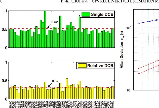
Fig. 3. The standard deviations of the receiver DCBs derived from the GPS reference stations relative to the mean (in DCB). The upper panel shows the standard deviations obtained from the single DCB estimation method, and the lower panel shows those by the relative DCB estimation method. The red dashed-dot lines represent the mean values of the standard deviations.
Fig. 4. The hourly receiver DCB values estimated using the data recorded from two GPS sites (BHAO and CHNG) for March 3–9, 2011.
To assess the short term stability of the receiver DCB values obtained from the different methods, the hourly re-ceiver DCBs are estimated for March 3–9, 2011. Figure 4 shows two receiver DCB values estimated by the different approaches for these 7 days. We plotted the results obtained from two GPS sites (BHAO and CHNG) located in South Korea. The results derived from the single DCB method re-vealed a short-term instability on an hourly basis compared with the relative DCB method. The hourly variation of re-ceiver DCBs estimated by the single method is significantly higher. However, there is no difference between the single DCB and the relative DCB estimation approaches with re-spect to the mean value for the 7 days. It can be clearly ob-served that the relative estimation approach provides more stable receiver DCB values. These results are consistent with the results in Fig. 3. Figure 5 shows Allan
devia-Fig. 5. Allan deviations of the hourly receiver DCB values for two GPS sites (BHAO and CHNG) computed by different methods.
Fig. 6. Comparison of the receiver DCBs estimated by the IGS with those obtained from the KASI using DAEJ GPS data. TheX-axis denotes the chosen date, and theY-axis range is set from 0 to 25 ns.
tions of the hourly receiver DCB values for two GPS sites (BHAO and CHNG) computed by different methods. The blue lines in Fig. 5 refer to the single estimation approach, whereas the red-dot lines are obtained from the relative es-timation approach. For short time intervals, up to two or three hours, the Allan deviation between the single DCB and the relative DCB showed a large difference. For longer time intervals, the difference between both approaches was smaller. This might explain that the hourly receiver DCB values computed by the single estimation have a higher vari-ability. Although the single estimation approach revealed a short-term instability, it can undoubtedly produce a receiver DCB of good accuracy, whether daily or long term.
As a result, if a receiver DCB is exactly known as a reference, the relative DCB estimation approach can give more stable information over a short-term period.
compari-son of receiver DCBs estimated by IGS as a reference with those obtained from the Korea Astronomy and Space Sci-ence Institute (KASI) using DAEJ GPS data. The X-axis denotes the dates and theY-axis range is set from 0 to 25 ns. The KASI has directly computed the daily receiver DCB values using the single receiver DCB estimation approach. The IGS DCB values were obtained from IGS GIMs. As observed in Fig. 6, the difference of daily receiver DCBs estimated by the IGS and KASI is less than 0.3 ns for 7 days. The corresponding RMS value is approximately 0.18 ns. Therefore, it is obvious that there is little difference be-tween the IGS DCB and the KASI DCB obtained from the single receiver DCB approach.
From the results derived from the single DCB estimation, it can be observed that the variation of daily receiver DCBs was also quite stable within the 7 days that were chosen for analysis.
4.
Summary
Two approaches for receiver DCB estimation have been suggested: One is to use a GPS network and the other is to calculate the DCB from a single receiver only. For comparison, we processed the GPS data obtained from the Korean GPS and compared the results estimated by the different methods. From the results of Figs. 1 and 2, the daily averaged receiver DCB values obtained from the two different approaches were in good agreement. The RMS value of those differences for all GPS sites is less than 1 ns. For a detailed comparison of both approaches, the vari-ability of the hourly estimated receiver DCB values was ex-amined by the standard deviation. The standard deviation of the receiver DCBs estimated by the relative DCB tion is less than that in the case of the single DCB estima-tion. The mean values of the standard deviations obtained from the relative and single methods are approximately 0.32 and 0.50, respectively. From this analysis, it is clear that the relative DCB estimation approach can obtain more stable values compared with the single DCB estimation approach in the short term.
In addition, to assess the short-term variability of the re-ceiver DCB values obtained from the different methods, the hourly receiver DCBs were estimated for March 3–9, 2011. The results derived from the single DCB method showed a short-term instability on an hourly basis, compared with the relative DCB method. It can be clearly observed that the relative DCB estimation approach provides more sta-ble receiver DCB values over the short term. However, the single DCB estimation approach can also produce a good daily averaged DCB accuracy over longer periods of time. Our results indicate that an appropriate combination of both methods can provide the best solution for receiver DCB es-timation.
In addition, the comparison between the DCB value ob-tained by the KASI and that of the IGS GIMs showed a good agreement at the level of 0.3 ns for the 7 days. The corresponding RMS value was 0.18 ns. Because the racy of the estimated DCBs significantly affects the accu-racy of ionospheric TEC estimation, ensuring the reliability of estimated DCBs is crucial.
Acknowledgments. We appreciate the Referee’s critical com-ments which were helpful in improving our manuscript. This work has been supported by the KASI’s basic core technology fund in 2011.
References
Choi, B. K., J. Cho, and S. Lee, Estimation and analysis of GPS receiver differential code biases using KGN in Korean Peninsula,Adv. Space Res.,47, 1590–1599, 2011.
Coco, D., C. Coker, S. Dahlke, and J. Clynch, Variability of GPS satellite differential group delay biases,IEEE Trans. Aero. Elec. Sys.,27, 931– 938, 1991.
Davies, K. and G. K. Hartmann, Studying the ionosphere with the Global Positioning System,Radio Sci.,32(4), 1695–1703, 1997.
Feltens, J. and N. Jakowski, The International GPS Service (IGS) iono-sphere working activity,SCAR Rep.,21, 2002.
Gao, Y. and Z. Liu, Precise ionosphere modeling using regional GPS network data,J. GPS,1, 18–24, 2002.
Grejner-Brzezinska, D., P. Wielgosz, I. Kashni, D. A. Smith, P. Spencer, S. Robertson, and G. L. Mader, An analysis of the effects of different network-based ionosphere estimation models on rover positioning ac-curacy,J. GPS,3, 115–131, 2004.
Hernandez-Pajares, M., J. Juan, and J. Sanz, New approaches in global ionospheric determination using ground GPS data,J. Atmos. Sol. Terr. Phys.,61, 1237–1247, 1999.
Hernandez-Pajares, M., J. M. Juan, J. Sanz, R. Orus, A. Garcia-Rigo, J. Feltens, A. Komjathy, S. C. Schaer, and A. Krankowski, The IGS VTEC maps: A reliable source of ionospheric information since 1998,J. Geod., 83, 263–275, 2009.
Lanyi, G. E. and T. Roth, A comparison of mapped and measured total ionospheric electron content using global positioning system and bea-con satellite observation,Rado Sci.,23, 483–292, 1988.
Ma, G. and T. Maruyama, Derivation of TEC and estimation of instru-mental biases from GEONET in Japan,Ann. Geophys.,21, 2083–2093, 2003.
Ma, X., T. Maruyama, G. Ma, and T. Maruyama, Determination of GPS re-ceiver differential biases by neural network parameter estimation,Radio Sci.,40, doi:10.1029/2004RS003072, 2005.
Mannucci, A. J., B. D. Wilson, D. N. Yuan, C. H. Ho, U. J. Lindqwister, and T. F. Runge, A global mapping technique for GPS-derived iono-spheric total electron content measurements,Radio Sci.,33, 565–582, 1998.
Mannucci, A. J., B. A. Iijima, L. Sparks, X. Pi, B. D. Wilson, and U. J. Lindqwister, Assessment of global TEC mapping using a three-dimensional electron density model,J. Atmos. Sol. Terr. Phys., 61, 1227–1236, 1999.
Meza, A., Three dimensional ionospheric models from earth and space based GPS observations, Ph.D. thesis, Universidad Nacional de La Plata, 1999.
Otsuka, Y., T. Ogawa, A. Saito, T. Tsugawa, S. Fukao, and S. Miyazaki, A new technique for mapping of total electron content using GPS network in Japan,Earth Planets Space,54, 63–70, 2002.
Sardon, E. and N. Zarraoa, Estimation of the total electron content using GPS data: How stable are the differential satellite and receiver instru-mental biases?,Radio Sci.,32(5), 1899–1910, 1997.
Sardon, E., A. Rius, and N. Zarraoa, Estimation of the transmitter and receiver differential biases and the ionospheric total electron content from Global Positioning System observations,Radio Sci.,29(3), 577– 586, 1994.
Schaer, S., G. Beulter, and M. Rothacher, Mapping and predicting the iono-sphere, inProceedings of the IGS AC Workshop, Darmstadt, Germany, 1998.
Wilson, B. and A. Mannucci, Extracting ionospheric measurements from GPS in the presence of Anti-Spoofing, inProceedings of the ION GPS-94, 1599–1608, 1994.
Zhang, W., D. H. Zhang, and Z. Xiao, The influence of geomagnetic storms on the estimation of GPS instrumental biases,Ann. Geophys.,27, 1613– 1623, 2009.
Zhang, D. H., W. Zhang, Q. Li, L. Q. Shi, Y. Q. Hao, and Z. Xiao, Accuracy analysis of the GPS instrumental bias estimated from observations in middle and low latitudes,Ann. Geophys.,28, 1571–1580, 2010.