A new technique for mapping of total electron content
using GPS network in Japan
Y. Otsuka1, T. Ogawa1, A. Saito2,3, T. Tsugawa4, S. Fukao5, and S. Miyazaki6
1Solar-Terrestrial Environment Laboratory, Nagoya University 2School of Electrical and Computer Engineering, Cornell University 3On leave from Department of Geophysics, Graduate School of Science, Kyoto University
4Department of Geophysics, Graduate School of Science, Kyoto University 5Radio Science Center for Space and Atmosphere, Kyoto University
6Geographical Survey Institute
(Received October 31, 2000; Revised December 7, 2001; Accepted December 7, 2001)
The dual frequency radio signals of the Global Positioning System (GPS) allow measurements of the total number of electrons, called total electron content (TEC), along a ray path from GPS satellite to receiver. We have developed a new technique to construct two-dimensional maps of absolute TEC over Japan by using GPS data from more than 1000 GPS receivers. A least squares fitting procedure is used to remove instrumental biases inherent in the GPS satellite and receiver. Two-dimensional maps of absolute vertical TEC are derived with time resolution of 30 seconds and spatial resolution of 0.15◦×0.15◦ in latitude and longitude. Our method is validated in two ways. First, TECs along ray paths from the GPS satellites are simulated using a model for electron contents based on the IRI-95 model. It is found that TEC from our method is underestimated by less than 3 TECU. Then, estimated vertical GPS TEC is compared with ionospheric TEC that is calculated from simultaneous electron density profile obtained with the MU radar. Diurnal and day-to-day variation of the GPS TEC follows the TEC behavior derived from MU radar observation but the GPS TEC is 2 TECU larger than the MU radar TEC on average. This difference can be attributed to the plasmaspheric electron content along the GPS ray path. This method is also applied to GPS data during a magnetic storm of September 25, 1998. An intense TEC enhancement, probably caused by a northward expansion of the equatorial anomaly, was observed in the southern part of Japan in the evening during the main phase of the storm.
1.
Introduction
The dual frequency radio signals of the Global Position-ing System (GPS) at an altitude of 20,200 km allow the mea-surement of the total number of free electrons, called total electron content (TEC), along ray path from GPS satellite to receiver. This TEC, however, usually includes instrumen-tal biases inherent in the GPS receivers and transmitters. These biases must be removed to obtain absolute values of TEC. Several techniques to calculate absolute TEC using the Kalman filter have been proposed. Sard´onet al. (1994) estimated absolute TEC assuming that vertical TEC distri-bution is spatially linear around the zenith of the receiver. Bishop et al. (1996) developed a self-calibration of pseu-dorange errors (SCORE) technique which was validated by independent measurements (Bishopet al., 1997) and mod-eling (Luntet al., 1999a). These techniques can be applied for data from a single GPS receiver. Mannucciet al.(1998) produced global maps of vertical TEC by interpolating TEC of more than 60 worldwide GPS stations in order to study
∗Present address: 3-13 Honohara, Toyokawa, Aichi 442-8507, Japan.
Copy right c The Society of Geomagnetism and Earth, Planetary and Space Sciences (SGEPSS); The Seismological Society of Japan; The Volcanological Society of Japan; The Geodetic Society of Japan; The Japanese Society for Planetary Sciences.
a global distribution of TEC under magnetically disturbed conditions. Hoet al. (1996), using such global TEC maps, found significant TEC increases in the winter hemisphere during a magnetic storm. Buonsanto et al. (1999) com-pared global TEC maps with incoherent scatter radar data from Sondrestrom, Millstone Hill, Arecibo, and Jicamarca to study the May 1–5, 1995 storm event.
The Geographical Survey Institute (GSI) of Japan has launched its nationwide GPS array project in April 1994 and has installed more than 1000 receivers in Japan, called GPS Earth Observation Network (GEONET) (Miyazaki et al., 1997). The average distance between two receivers is approximately 25 km. One GPS receiver measures signals simultaneously from typically 6–7 satellites. GPS data are sampled every 30 seconds. These conditions allow the re-trieval of TEC maps over Japan with high spatial resolution and a time resolution of 30 seconds. The above-mentioned techniques to obtain absolute TEC are not applicable to GEONET data gathered from a large number of receivers, because it takes much computation time to use the Kalman filter for each update epoch.
In the present study, we develop a new simple and ro-bust technique to derive two-dimensional map of absolute TEC over Japan by using the GEONET data. This method provides absolute TEC as a function of time and location.
Simulated observations of TEC along ray paths from GPS satellites are used to validate this technique. The results are compared with MU radar observations under geomagneti-cally quiet conditions.
2.
Estimation of Absolute TEC and Instrumental
Biases
GPS observations provide both carrier phase delaysLand pseudorangesPof the dual frequencies (f1=1575.42 MHz
and f2 = 1227.60 MHz). Phase and group delays of radio
waves in the ionosphere,dpanddg(in meters), respectively, are proportional to total electron content integrated along propagation path,T (in electrons per square meter)
−dp=dg = 40.3T
f2 (1)
where f is the radio wave frequency in Hertz (e.g., Davies, 1990). Since the neutral gas influence on the refractive index is non-dispersive and does not depend on frequency, TEC can be derived by comparing the phase delays ofL1andL2
signal. 1 ns of differential time delay corresponds to 2.852 TEC units (TECU) where 1 TECU=1×10¹⁶electrons/m2. The difference of the carrier phase delays LI = L1 −L2
tracks very precisely TEC. However, sudden LI changes (cycle slip) sometimes occur when a GPS receiver losses lock on the GPS signals. The cycle slips are detected as discontinuity inLI and corrected using an algorithm devel-oped by Belwitt (1990). Although TEC derived from the phase data provides relative change of TEC, a level of TEC is unknown because of unknown initialization constant in phase data. Therefore, the level of TEC is adjusted to that of TEC derived from the corresponding pseudorange differ-ence (P2− P1) for each satellite-receiver pair. The level
is determined for each set of connected TECs. TEC data separated over more than 15 minutes in time are not con-nected. The pseudorange delays still contain delays inher-ent in satellite and receiver hardwares. To get absolute TEC, these biases must be removed.
As described above, absolute TEC, Ii(t), measured by satellite-i at epoch timetis determined from the phase and pseudorange data. Ii(t) consists of both the slant TEC,
Ti(t), along a satellite-receiver ray path and the instrumental biasBi.
Ii(t)=Ti(t)+Bi (2)
The instrumental biases are considered to be constant over several days (Sard´on et al., 1994; Sard´on and Zarraoa, 1997). We assume that the ionosphere is a thin shell. The thin-shell model assumption is commonly used in GPS TEC studies (e.g., Bishopet al., 1997; Sard´onet al., 1994). From this assumption, the slant TEC,Ti(t), at a give point in the ionospheric shell is related to the equivalent vertical TEC,
Vi(t), at that point by
Ti(t)=S(i(t))Vi(t) (3)
whereS(i(t))is the slant factor andi(t)is the elevation angle of the GPS satellite. ThusIi(t)is written as follows:
Ii(t)=S(i(t))Vi(t)+Bi (4)
The ionization distribution is approximated by a slab of constant-density with the lower and upper boundary at alti-tudes of 300 and 550 km, respectively. Then, the slant factor
S is defined asS =τ1/τ0, whereτ1is the length of the ray
path between 300 and 550 km altitudes andτ0is the
iono-sphere thickness of 250 km for zenith path. However, actual electron density distribution is not so simple as this assump-tion and extends toward higher (the plasmasphere) and lower (the E region) altitudes. The assumption, therefore, causes some errors in the estimation of vertical TECs. The error increases with increasing slant factor S at lower elevation angle. For example,Sis 1.73 at elevation angle of 30◦. For this reason, data with elevation angles less than 30◦are ex-cluded in our method.
The procedure to construct a two-dimensional map of absolute vertical TEC with high time and spatial resolution consists of the following three steps. First, hourly averages of TEC are estimated by applying a weighted least squares fitting procedure to the GPS data from a single receiver. Next, the instrumental biases are determined by using the hourly TEC average that is obtained in the first step. Finally, the biases are removed from the measured TEC to derive absolute TECs. Two-dimensional maps of absolute vertical TEC with a time resolution of 30 seconds and a spatial resolution of 0.15◦ ×0.15◦ in latitude and longitude are constructed through these steps. We describe the detailed procedures in these steps below.
(1) Estimation of hourly TEC average: Equation (4) is
divided byS(i)and averaged over one hour to estimate the hourly TEC average. Here, we assume that the hourly aver-age of vertical TEC is uniform within an area covered by a receiver; this area approximately corresponds to a surround-ing of 1000 km. This assumption means that the hourly ver-tical TECs obtained from different satellite links by one re-ceiver are the same and can be averaged to a value of vertical
TEC,Vk, for each timekwherekdenotes the index of time
sequence of hourly TEC average. Thus, the following equa-tion is derived from Eq. (4).
Ik/S(ki)=Vk+1/S(ik)B
i (5)
fork =1,2, . . . ,Nt andi =1,2, . . . ,Ns whereNt is the number of hourly TEC average, and Ns is the number of satellites which are observed by one receiver. Here, vari-ables with overline denote averaged values.
The number of equations is usually larger than that of the unknowns (Vkwithk = 1,2, . . . ,Nt and Bi withi = 1,2, . . . ,Ns). The unknowns are determined through a least squares fitting procedure minimizing the following residual:
E =
Ns
i
Nt
k
Wki
Ik/S(ik)−(Vk+1/S(ki)B
i)2 (6)
where Wi
factor:
Wki =1/S(i
k) (7)
Wkibecomes smaller with decreasing elevation angle. Since the GPS satellites appear over a fixed receiver every about 24 hours, our procedure requires continuous data over more than 24 hours at the receiver. In the present study, we use a data set consisting of 24-hour data (Nt =24). This proce-dure is applied to the GPS data from the GEONET consist-ing of more than 1000 receivers. We derive more than 1000 data sets of the hourly TEC averages (Vk,k=1,2, . . . ,Nt) and the instrumental biases (Bi,i =1,2, . . . ,N
s).
(2) Estimation of instrumental biases:Hourly TEC
av-erages are mapped on the ionospheric shell which is as-sumed to be located at 400 km altitude. Since the receivers are closely distributed (average distance between two re-ceivers is about 25 km), areas where different rere-ceivers pro-vide TEC estimates overlap. These overlapped TECs are smoothed to obtain the hourly TEC averages within a loca-tion of 1◦×1◦ in latitude and longitude. This smoothing suppresses isolated outliers and reduces estimation errors of the hourly TEC average derived from the least squares fitting procedure. Substituting the hourly average and spa-tially smoothed TECs into Eq. (5) determines the instrumen-tal biasesBi. This newBi is more accurate due to spatially smoothing of the hourly TEC averages than the previousBi derived by the least square fitting procedure in step (1).
(3) Mapping of absolute TEC: Substituting Bi into
Eq. (4) gives vertical TEC,Vi(t), at a sampling interval of
t(30 seconds). Absolute vertical TECVi(t)are mapped on the ionospheric shell at the 400 km altitude with a pixel of 0.15◦ ×0.15◦ in latitude and longitude. Vi(t)within one pixel are averaged. Thus, two-dimensional maps of vertical TEC with a spatial resolution of 0.15◦×0.15◦ in latitude and longitude are derived every 30 seconds.
This technique to derive absolute TEC uses data from a large number of closely-distributed GPS receivers and does not need interpolation of TEC in space and time. This tech-nique is also applicable to data from a single receiver. In this case, however, two-dimensional maps of TEC are not obtained because of scarcity of TEC distribution. Only a dense distribution of GPS receivers, such as GEONET, pro-vides two-dimensional map of absolute TEC as a function of location and time.
3.
Validation of the Method
3.1 Model simulation
We have examined the expected accuracy of this tech-nique using computer simulations. To simulate actual mea-surements of TEC observed at ground GPS stations in Japan, we use a model for electron contents based on the Interna-tional Reference Ionosphere (IRI-95) model (Bilitza, 1990) and the results of the Sheffield University Plasmasphere and Ionosphere Model (SUPIM) (Balanet al., 2002). The elec-tron contents in the altitude range of 100–1,000 km are taken from the 95 model. The electron content from the IRI-95 varies with altitude, local time, latitude and longitude.
Electron contents above 1,000 km altitude are extrapo-lated to match the results reported by Balanet al. (2002).
(a)
0 6 12 18 24
UT (JST 9hours) 0
10 20 30 40 50 60 70 80 90 100
Vertical TEC [10
16 m 2 ]
[43oN, 143oE]
(b)
0 6 12 18 24
UT (JST 9hours) 0
10 20 30 40 50 60 70 80 90 100
Vertical TEC [10
16 m 2 ]
[38oN, 140oE]
(c)
0 6 12 18 24
UT (JST 9hours) 0
10 20 30 40 50 60 70 80 90 100
Vertical TEC [10
16 m 2 ]
[33oN, 131oE]
Table 1. Accuracy of the estimation procedure.
Location 1 Location 2 Location 3
[43◦N, 143◦E] [38◦N, 140◦E] [33◦N, 131◦E]
Solar maximum equinox −2.0±0.1 TECU −2.5±1.4 TECU −1.9±2.7 TECU
Solar maximum winter −0.4±0.9 TECU 0.0±1.6 TECU 2.0±2.9 TECU
Solar maximum summer −2.8±0.6 TECU −2.8±0.9 TECU −2.9±1.7 TECU
Solar minimum equinox −0.6±0.5 TECU −1.5±1.3 TECU −2.6±2.3 TECU
Solar minimum winter −0.6±0.5 TECU −0.9±0.8 TECU −0.8±1.3 TECU
Solar minimum summer −0.6±0.3 TECU −1.2±0.6 TECU −2.3±1.5 TECU
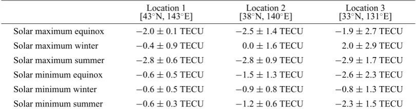
Averages and standard deviations of difference between the estimated vertical TEC and the corresponding vertical TEC given by the model based on the IRI-95 model over three locations for three seasons under solar maximum and minimum conditions.
They have presented vertical electron content profiles cal-culated by SUPIM up to the GPS altitude (about 20,200 km) at noon and midnight in winter, summer and equinox. They have also shown that plasmaspheric electron content changes appreciably with season and latitude but very little with local time. These variations of plasmaspheric electron content are replicated in our model.
Ephemerides of the satellites are chosen to correspond to those of actual configurations of the GPS satellite on a par-ticular day. Slant electron contents are calculated along all ray paths between satellites and receivers with elevation an-gles above 30◦at an interval of 30 seconds. Arbitrary offsets which represent the unknown instrumental biases inherent in GPS satellite and receiver are added to the electron contents calculated from the model. The satellite (receiver) biases which differ for each satellite (receiver) are determined to lie within−10 to 20 (−50 to 50) TECU. The simulated GPS observations are reprocessed in the procedure described in Section 2 for the three seasons (equinox, winter, summer) under solar maximum and minimum conditions.
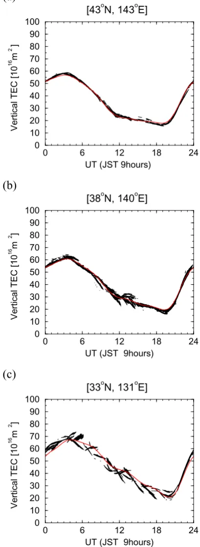
The simulation results in the case of solar maximum equinox are presented in Fig. 1. The figure shows diurnal variation of TEC over three locations. The red curves repre-sent the vertical TEC derived from integration of the model electron density between 100 and the GPS altitude of 20,200 km, which is input for the estimation procedure. The dotted points show the resultant TEC output from the estimation procedure within a range 1◦×1◦in longitude and latitude centered at the ground station at an interval of 30 seconds. The segments of the TEC curve relate to ray paths from individual satellites. The scatter of estimated TEC reflects imperfection in the estimation procedure. The difference between the input and output increase with decreasing lat-itude: the difference is less than 2 TECU at 43◦N while it is around 5 TECU at 33◦N. This fact can be explained in terms of the extent of the area covered by a GPS receiver. Since the GPS satellite is in an orbit with inclination of 55◦, the area covered with a GPS receiver is wider at low latitudes than at high latitudes. In the procedure estimating absolute TEC, the homogeneity in the area covered by a GPS receiver is assumed. Thus, the discrepancy from this assumption is more severe with decreasing latitude.
The differences between the estimated vertical TEC and
the corresponding vertical TEC given by the model are cal-culated at three locations for three seasons under solar max-imum and minmax-imum conditions. The average and standard deviation of these differences during the 24-hour period are listed in Table 1. Most averages are negative, which means underestimation of vertical TEC. This underestimation is qualitatively explained in terms of inaccuracy of the thin-shell model assumption. To define the slant factor, we ap-proximate the plasma distribution by a constant-density slab with lower and upper boundaries at 300 and 550 km alti-tudes, respectively. However, the actual plasma distribution extends toward the plasmasphere. Here, we compare the slant factors for the ionosphere and the plasmasphere. The slant factor at altitudeh, which is defined as inverse of co-sine of satellite zenith angle at a subionospheric point, is given as follows:
S()= 1
cosarcsin RR+hcos() (8)
whereis the elevation angle of the line-of-sight from the receiver to the satellite, andRis the radius of the Earth. At an elevation angle of 60◦ (30◦), S is 1.14 (1.73) and 1.02 (1.06) at 400 km and 10,000 km altitude, respectively; that is,S for the plasmasphere is smaller than that for the iono-sphere. The ratio between these two increases with decreas-ing elevation angles and reaches 0.6 at elevation angle of 30◦. This causes overestimation of the slant factor. As a result, the equivalent vertical TEC, to which the slant TEC is converted by dividing the slant factor, is underestimated. The underestimation is largest for the solar maximum sum-mer condition, for which the plasmaspheric electron content is highest. From Table 1, it is found that the estimated TEC is less than TEC integrated up to the GPS altitude of 20,200 km; the difference is less than 3 TECU. The standard devi-ation of the difference between the two is less than 1 TECU (3 TECU) at the northern (southern) part of Japan.
The slant factor at an elevation angle of 45◦ decreases by 2% when the slab altitude increases by 200 km. The de-crease of the slant factor becomes smaller for smaller zenith angle. Therefore, we conclude that the altitude change of the F layer does not cause significant errors in estimating absolute TEC.
Latitudinal variation of the plasmaspheric electron con-tent also limits accurate determination of vertical TEC from GPS data. Lunt et al. (1999a) have showed that vertical TEC estimated on ray paths to the south of the European mid-latitude station exceeds that on ray paths to the north by an average of 0.7 TECU. Accurate estimation of vertical TEC requires to know the plasmaspheric electron content distribution.
It is concluded from the present model simulation that our TEC estimation procedure may underestimate actual TEC by less than 3 TECU. The magnitude of underestimation mainly depends on the plasmaspheric electron content. The estimated TECs scatter with the standard deviation of less than 1 TECU (3 TECU) at the northern (southern) part of Japan. It should be noted that these errors are mainly caused by the two assumptions; one is the thin-shell model assump-tion and the other is the homogeneity of vertical TEC in the area covered with a GPS receiver.
3.2 Comparison with MU radar observations
To validate this estimation method of vertical TEC over Japan, the estimated absolute GPS TECs are compared with the incoherent scatter MU radar observations. The MU radar is located at Shigaraki (34.85◦N, 136.10◦E). Details of the MU radar system have been described by Fukaoet al. (1985a, b). Altitude profiles of the electron density are obtained from power profile measurements of the incoher-ent echoes from the ionospheric electrons. A pulse width of 512μs is used to maximize signal-to-noise ratio. For this long-pulse measurement, the signal-to-noise ratio is larger than unity over a considerable altitude range around theF2 peak altitude. The received power profiles are integrated to form hourly profiles. The number of integration is approxi-mately 240,000, yielding random statistical errors of the sig-nal power less than 1% around the F2 peak altitude. The received power profiles are corrected for range dependence and electron-ion temperature ratio. The temperature ratio is taken from a model based on the MU radar observations dur-ing the period from 1986 to 1997 (Otsukaet al., 1998). The resulting power profiles are normalized to theF2 layer peak density using critical frequency for theF2 layer, foF2, ob-tained from an ionosonde at Kokubunji (35.7◦N, 139.5◦E) to produce the electron density profiles. The electron density observed with the MU radar is integrated from 100 km to 1,000 km altitude to obtain vertical TEC. Since the random statistical error of the MU radar signal is less than 1%, the expected error of TEC is determined mainly by the resolu-tion of foF2 (0.1 MHz). foF2 is 7–8 MHz during daytime and 4–6 MHz during nighttime for the period of May 6–8, 1998. The error of MU radar TEC is thus 2–5%.
The estimated vertical GPS TECs from the GEONET are compared to TECs derived from the MU radar observations. Figure 2 shows temporal variations of the GPS and MU radar vertical TECs over the MU radar for three consecutive days, May 6–8, 1998. The geomagnetic conditions were
(a)
09 12 15 18 21 00 03 06 09
Local time (hours) 5
10 15 20 25 30
Vertical TEC [10
16 m -2 ]
May 6, 1998
GPS MU
(b)
09 12 15 18 21 00 03 06 09
Local time (hours) 5
10 15 20 25 30
Vertical TEC [10
16 m -2 ]
May 7, 1998
GPS MU
(c)
09 12 15 18 21 00 03 06 09
Local time (hours) 5
10 15 20 25 30
Vertical TEC [10
16 m -2 ]
May 8, 1998
GPS MU
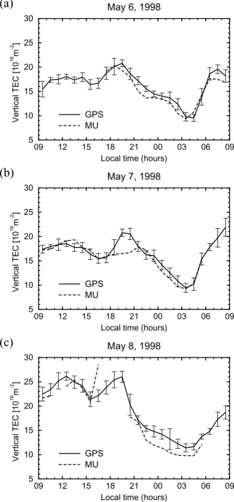
Fig. 2. Comparison of diurnal variations of TEC over Shigaraki derived from GPS GEONET and from MU radar observations on (a) May 6, (b) May 7, and (c) May 8, 1998. The GPS TEC is averaged over one hour within the area of 1◦×1◦in longitude and latitude centered at the MU radar. The error bar shows its standard deviation. The MU radar TEC is obtained by integrating electron density from 100 to 1,000 km altitude.
from other radio sources.
As shown in Fig. 2, both the GPS and MU radar TECs decrease from a maximum after sunset, reach a minimum just before sunrise, and then increase in the morning. It is obvious that diurnal and day-to-day variations of the GPS TEC are similar to those of the MU radar TEC, although the GPS TEC magnitude exceeds the MU radar TEC by 2 TECU on average. The difference is considered to represent the plasmaspheric TEC because the GPS altitude is about 20,200 km while the MU radar TEC is derived from the in-tegration up to 1,000 km altitude. It should be noted that the TEC is underestimated by about 1–2 TECU in the solar min-imum summer (Table 1). Therefore, the plasmaspheric TEC is about 3–4 TECU on average. This value is slightly larger than the plasmaspheric TEC estimated at mid-latitudes in the European and American sectors by Luntet al. (1999b). This difference is due to the latitudinal variation of plasma-spheric electron content. According to Luntet al. (1999b), the plasmaspheric electron content in the European sector is 2 TECU at the solar minimum while the corresponding value in the American sector is about 0.5 TECU. Balanet al.
(2002) have obtained the plasmaspheric electron contents over Japan by comparing TEC obtained from the GEONET with that derived from SUPIM for different seasons at high solar activity. According to their study, the plasmaspheric contribution to the GPS TEC is up to 12 TECU at high solar activity, which changes appreciably with season and latitude and very little with the time of day.
A large difference between the two TECs occurs during 19–23 LT on May 7 (Fig. 2). In this period, southwestward-propagating traveling ionospheric disturbances (TIDs) with a wavelength of several hundred kilometers and an ampli-tude of approximately 1 TECU were observed. It is noted that spatial variation (less than 1,000 km) of TEC induced by TIDs may cause estimation errors of the GPS TEC to a certain degree because our method assumes that TEC is uni-form within the area covered by a receiver. Ogawaet al.
(2002) have studied TIDs using vertical GPS TEC data and find a coincidence of TID-related structures in TEC and 630-nm airglow intensity. They show that fluctuation amplitudes of TEC are 0.5–2.5 TECU (relative amplitudes of a few to 20%).
The discrepancy between the two TEC also occurs at 16 LT on May 8. The MU radar TEC increases more rapidly than the GPS TEC, and exceeds the GPS TEC by 5 TECU. This situation is physically impossible. The most possible explanation is that electron density profile observed with the MU radar is contaminated by interferences from other radio sources or coherent echoes which return from field-aligned irregularities embedded in sporadic E layers through the antenna sidelobes (e.g., Yamamotoet al., 1991, 1992); the contamination causes overestimate of the MU radar TEC. Intense echoes which are expected to come from the field-aligned irregularities are received during 17–19 LT on May 8, so that the MU radar TEC is lost during this period.
From comparison between Fig. 2(a), (b), and (c), it is found that differences between GPS TEC and MU radar TEC tend to increase day by day. This indicates increase of the plasmaspheric electron content during this period. A geomagnetic storm occurred on May 4, 1998. Dst index
reached a minimum of−205 nT at 15 LT on May 4. A geo-magnetic storm causes rapid contraction of the plasmapause and depletion of the flux tubes around the dusk on the first day of the storm. A gradual replenishment of the plasma-spheric ionization from the underlying ionosphere then oc-curs for a period of many days after the storm (Kersleyet al., 1978; Kersley and Klobuchar, 1980). The period of May 6– 8, 1998 shown in Fig. 2 corresponds to that of replenishment of the plasmaspheric plasma. Kersley and Klobuchar (1980) have presented storm-associated depression and replenish-ment of plasmaspheric electron content using ATS 6 obser-vations, in which plasmaspheric electron content was pro-vided by the difference between TEC measured by a group delay technique and that from Faraday rotation. A rapid de-pression of 1–2 TECU was observed during the evening of the first day of the storm, followed by a gradual replenish-ment over many days up to the next storm. Similar behav-ior of the plasmaspheric electron content also has been ob-served with the Japanese geostationary satellite ETS-II for the geomagnetic storm on February 15–16, 1978 (Ogawaet. al., 1980). The depression of plasmaspheric electron content was about 5 TECU and its continuation is 1.5 days.
4.
Application of the method
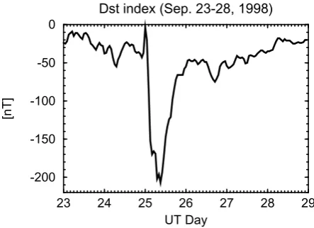
In order to demonstrate performance of two-dimensional map of absolute TEC obtained from a GPS network (GEONET) in Japan and its usefulness to the ionospheric study, especially geomagnetic storm effect on the iono-sphere, our method is applied to GPS data on a geomag-netic storm day, September 25, 1998. Figure 3 shows Dst
index during the period September 23–28, 1998. A sudden storm commencement occurred at about 00 UT (09 LT) on September 25, 1998. Dst reached a minimum of−207 nT at 09 UT (18 LT).
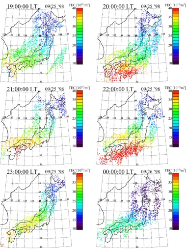
Figure 4 shows two-dimensional maps of vertical TEC over Japan at each hour during 19–24 LT on September 25, 1998. The data coverage is 30◦–46◦N in latitude and 128◦–146◦E in longitude. The time resolution is 30 seconds and the spatial resolution is 0.15◦ ×0.15◦ in latitude and longitude. A clear enhancement of TEC is seen during 19–
23 24 25 26 27 28 29 UT Day
-200 -150 -100 -50 0
[nT]
Dst index (Sep. 23-28, 1998)
Fig. 3. Dst index during September 23–28, 1998. A sudden storm commencement occurs at about 00 UT on September 25, 1998. Dst
128 130 132 134 136 138 140 142 144 146
19:00:00 LT
09/25 ’98128 130 132 134 136 138 140 142 144 146
30
128 130 132 134 136 138 140 142 144 146
30
20:00:00 LT
09/25 ’98128 130 132 134 136 138 140 142 144 146
30
128 130 132 134 136 138 140 142 144 146
30
21:00:00 LT
09/25 ’98128 130 132 134 136 138 140 142 144 146
30
128 130 132 134 136 138 140 142 144 146
30
22:00:00 LT
09/25 ’98128 130 132 134 136 138 140 142 144 146
30
128 130 132 134 136 138 140 142 144 146
30
23:00:00 LT
09/25 ’98128 130 132 134 136 138 140 142 144 146
30
128 130 132 134 136 138 140 142 144 146
30
00:00:00 LT
09/26 ’98128 130 132 134 136 138 140 142 144 146
30
Fig. 4. Two-dimensional maps of absolute vertical TEC over Japan during 19–24 LT on September 25.
23 LT. The TEC enhancement is more intense in southern part of Japan. This is possibly associated with a poleward expansion of the equatorial anomaly. The expansion is due to storm-related enhancements of eastward electric fields at the equatorial region which cause the equatorial fountain effect.
Ogawa et al. (1980) have reported a similar phenom-ena, in which storm-associated enhancements of foF2 and TEC over Japan were observed in the evening when horizon-tal component of geomagnetic field disturbances reached a minimum of−22 nT. The enhancement of foF2 was more severe and earlier in the southern part of Japan.
Buonsantoet al.(1999) have also shown a large increase
in foF2 observed at Arecibo during the first night of a geomagnetic storm (May 2, 1995). They have compared the results with the global maps of vertical TEC derived from GPS data and suggested that the TEC enhancement is associated with the poleward expansion of the equatorial anomaly.
5.
Summary
We have developed a new technique to estimate absolute values of vertical TEC over Japan using GEONET data. In this technique a weighted least squares fitting is used to determine instrumental biases, assuming that hourly TEC average is uniform within an area covered by a GPS receiver. Two-dimensional maps of absolute vertical TEC are derived with a time resolution of 30 seconds and a spatial resolution of 0.15◦×0.15◦in latitude and longitude. The method does not require interpolation between TEC measurements.
Accuracy of TEC estimated from our method has been investigated using model simulations. It is found that TEC is underestimated by less than 3 TECU. The amount of un-derestimation mainly depends on that of the plasmaspheric electron content. The estimated TECs scatter with standard deviations of less than 1 TECU (3 TECU) at the northern (southern) part of Japan. These errors are mainly caused by two assumptions, that is, thin-shell model assumption and the homogeneity of vertical TEC in the area covered with a GPS receiver.
The estimated vertical GPS TECs have been compared with ionospheric electron contents calculated from electron density profiles of the MU radar. Diurnal and day-to-day variations of the GPS TEC are reasonably in agreement with those of the ionospheric electron content although the GPS TECs are larger than the ionospheric contents by 2 TECU on average. This difference can be also attributed to the plas-maspheric electron content along GPS ray path. Compari-son between the GPS TEC and MU radar observations can yield storm-associated variations of the plasmaspheric elec-tron content. Two-dimensional maps of absolute GPS TEC have reveal TEC enhancements during the main phase of the storm on September 25, 1998. The enhancement is more in-tense in the southern part of Japan, and is possibly caused by an expansion of the equatorial anomaly due to an enhance-ment of eastward electric field in the equatorial region. Con-tinuous observations of absolute TEC over wide area with high temporal and spatial resolutions will contribute to more extensive study and monitoring of the ionosphere.
Acknowledgments. GEONET GPS data were provided by the Geographical Survey Institute of Japan. Ionograms at Kokubunji were provided by the Communications Research Laboratory, Tokyo. The MU radar is owned and operated by the Radio Sci-ence Center for Space and Atmosphere of Kyoto University. The authors would like to thank N. Balan and K. Shiokawa for their helpful comments and suggestions. This work was supported by Grand-in-Aid for Scientific Research of the Ministry of Education, Culture, Sports, Science and Technology of Japan (12554016).
References
Balan, N., Y. Otsuka, T. Tsugawa, S. Miyazaki, T. Ogawa, and K. Sh-iokawa, Plasmaspheric electron content in the GPS ray paths over Japan under magnetically quiet conditions at high solar activity,Earth Planets Space,54, this issue, 71–79, 2002.
Belwitt, G., An automatic editing algorithm for GPS data,Geophys. Res. Lett.,17, 199–202, 1990.
Bilitza, D. (Ed.), International Reference Ionosphere 1990,Rep. NSSDC, 90–22, National Space Science Center, Greenbelt, MD, 1990.
Bishop, G. J., A. Mazzella, E. Holland, and S. Rao, Algorithms that use the ionosphere to control GPS errors,in Proceedings of the IEEE 1996 Position Location and Navigation Symposium (PLANS)pp. 145–152, IEEE Press, Piscataway, N. J., 1996.
Bishop, G. J., D. S. Coco, N. Lunt, C. Coker, A. J. Mazzella, and L. Kersley, Application of SCORE to extract protonospheric electron content from GPS/NNSS observations,in Proceedings of ION GPS ’97,pp. 207–216, Inst. of Navig., Alexandria, Va., 1997.
Buonsanto, M. J., S. A. Gonz´alez, X. Pi, J. M. Ruohoniemi, M. P. Sulzer, W. E. Swartz, J. P. Thayer, and D. N. Yuan, Radar chain study of the May, 1995 storm,J. Atmos. Solar Terr. Phys.,61, 233–248, 1999. Davies, K., Ionospheric Radio, IEE Electromagnetic Waves Series, 31,
Peter Peregrinus, London, 1990.
Fukao, S., T. Sato, T. Tsuda, S. Kato, K. Wakasugi, and T. Makihira, The MU radar with an active phased array system, 1, Antenna and power amplifiers,Radio Sci.,20, 1155–1168, 1985a.
Fukao, S., T. Tsuda, T. Sato, S. Kato, K. Wakasugi, and T. Makihira, The MU radar with an active phased array system, 2, Inhouse equipment,
Radio Sci.,20, 1169–1176, 1985b.
Ho, C. M., A. J. Mannucci, U. J. Lindqwister, X. Pi, and B. T. Tsurutani, Global ionosphere perturbations monitored by the worldwide GPS net-work,Geophys. Res. Lett.,23, 3219–3222, 1996.
Kawamura, S., Y. Otsuka, S.-R. Zhang, S. Fukao, and W. L. Oliver, A climatology of middle and upper atmosphere radar observations of ther-mospheric winds,J. Geophys. Res.,105, 12,777–12,788, 2000. Kersley, L. and J. A. Klobuchar, Storm associated protonospheric depletion
and recovery,Planet. Space Sci.,28, 453–458, 1980.
Kersley, L., H. Hajeb-Hossienieh, and K. J. Edwards, Post-geomagnetic storm protonospheric replenishment,Nature,271, 429–430, 1978. Lunt, N., L. Kersley, G. J. Bishop, A. J. Mazzella, and G. J. Bailey, The
ef-fect of the protonosphere on the estimation of GPS total electron content: Validation using model simulations,Radio Sci.,34, 1261–1271, 1999a. Lunt, N., L. Kersley, and G. J. Bailey, The influence of the protonosphere on
GPS observations: Model simulations,Radio Sci.,34, 725–732, 1999b. Mannucci, A. J., B. D. Wilson, D. N. Yuan, C. H. Ho, U. J. Lindqwister, and
T. F. Runge, A global mapping technique for GPS-derived ionospheric total electron content measurements,Radio Sci.,33, 565–582, 1998. Miyazaki, S., T. Saito, M. Sasaki, Y. Hatanaka, and Y. Iimura, Expansion of
GSI’s nationwide GPS array,Bull. Geogr. Surv. Inst.,43, 23–34, 1997. Ogawa, T., K. Sinno, M. Fujita, and J. Awaka, Severe disturbances of VHF
and GHz waves from geostationary satellites during a magnetic storm,J. Atmos. Terr. Phys.,42, 637–644, 1980.
Ogawa, T., N. Balan, Y. Otsuka, K. Shiokawa, C. Ihara, T. Shimomai, and A. Saito, Observations and modeling of 630 nm airglow and total electron content associated with traveling ionospheric disturbances over Shigaraki, Japan,Earth Planets Space,54, this issue, 45–56, 2002. Otsuka, Y., S. Kawamura, N. Balan, S. Fukao, and G. J. Bailey, Plasma
temperature variations in the ionosphere over the middle and upper at-mosphere radar,J. Geophys. Res.,103, 20,705–20,713, 1998. Sard´on, E. and N. Zarraoa, Estimation of total electron content using GPS
data: How stable are the differential satellite and receiver instrumental biases?,Radio Sci.,32, 1899–1910, 1997.
Sard´on, E., A. Rius, and N. Zarraoa, Estimation of the transmitter and receiver differential biases and the ionospheric total electron content from Global Positioning System observations,Radio Sci.,29, 577–586, 1994.
Yamamoto, M., S. Fukao, R. F. Woodman, T. Ogawa, T. Tsuda, and S. Kato, Mid-latitudeE-region field-aligned irregularities observed with the MU radar,J. Geophys. Res.,96, 15,943–15,949, 1991.
Yamamoto, M., S. Fukao, T. Ogawa, and S. Kato, A morphological study of mid-latitudeE-region field-aligned irregularities revealed by the MU radar,J. Atmos. Terr. Phys.,54, 769–777, 1992.