R E S E A R C H
Open Access
Ultra-short-term wind speed forecasting
based on support vector machine with
combined kernel function and similar data
Jian He
*and Jingle Xu
Abstract
The accuracy of wind power prediction is very important for the stable operation of a power system. Ultra-short-term wind speed forecasting is an effective way to ensure real-time and accurate wind power prediction. In this paper, a short-term wind speed forecasting method based on a support vector machine with a combined kernel function and similar data is proposed. Similar training data are selected based on the wind tendency, and a combination of two kinds of kernel functions is applied in forecasting using a support vector machine. The forecasting results for a wind farm in Ningxia Province indicate that a combination of kernel functions with complementary advantages outperforms each single function, and forecasting models based on grouped wind data with a similar tendency could reduce the forecasting error. Furthermore, more accurate wind forecasting results ensure better wind power prediction.
Keywords:Wind power, Ultra-short-term speed forecasting, Support vector machine, Compound kernel function,
Similar data
1 Introduction
As environmental issues have become more prominent, wind power has been rapidly developing as a clean renewable energy source [1–3]. In recent years, the single-unit capacity of wind turbines and the total power generation capacity of large-scale grid-connected wind farms have grown rapidly, and the impact on power systems is becoming increasingly obvious. In some cases, the safety of conventional power systems may even be compromised [2]. Accurate prediction of the power generation of wind farms is a necessary means to improve the operational stability of power systems. Since the output power of a wind turbine is directly dependent on the actual wind speed, a research hotspot is to realize wind power prediction indirectly through wind speed prediction [3–6].
Currently used wind speed prediction methods usually include continuous methods [7], Kalman filters [8, 9], random time series [10–13], neural network methods [14–19], spatial correlation methods [20, 21], flow field
precalculation (CFD)-based methods [21], Adaboost-based approaches [22], and support vector machines [23–25]. The literature [26] proposed a multi-layer feed-forward (BP) neural network wind speed prediction method based on similarity curve samples. Although this neural network method has good prediction effects in many fields, it has the disadvantages of local minimization and slow convergence. In [25], a support vector machine based on a wavelet kernel function is proposed and not only has the advantages of local analysis and feature extraction for non-stationary signals but can also approximate any non-linear function in the extended space. Since each kind of kernel function has its own advantages, increasing attention has been paid to combin-ing two or more kinds of kernel functions to improve the performance of the model [27,28].
For the prediction of ultra-short-term wind speed, this paper proposes a support vector machine prediction model based on a combined kernel function and similar data. In this model, the training samples are extracted based on the trend of changes in wind speed, and a training model is established. A combination of two kinds of kernel functions is used to construct the
© The Author(s). 2019Open AccessThis article is distributed under the terms of the Creative Commons Attribution 4.0 International License (http://creativecommons.org/licenses/by/4.0/), which permits unrestricted use, distribution, and reproduction in any medium, provided you give appropriate credit to the original author(s) and the source, provide a link to the Creative Commons license, and indicate if changes were made.
* Correspondence:[email protected]
support vector machine to realize the ultra-short-term prediction of wind speed. The wind speed data predic-tion based on a wind field in Ningxia shows that the combination of a wavelet kernel function and polyno-mial kernel function has higher prediction accuracy than the single kernel functions. By predicting the training data independently according to similarity, the predic-tion is based on similarity. The predicpredic-tion error is further reduced. The wind turbine power calculated by the wind speed predicted by this method is very close to the actual output power of the wind turbine.
2 Wind speed prediction by support vector machine based on combined kernel function and similar data
2.1 Common support vector machine kernel functions Support vector machine is a machine learning method based on statistical theory. It maps the input sample space to a high-dimensional linear feature space through a non-linear kernel function and has a good ability to deal with nonlinear regression problems. For an SVM model, the choice of kernel function has an important impact on the performance of the model. There are four common SVM (support vector machine) kernel func-tions. Equations (1), (2), and (3) are traditional kernel functions, which are a linear kernel function, polynomial kernel function, and radial basis kernel function. Equa-tion (4) is a wavelet kernel funcEqua-tion.
K xi;xj
2.2 Combined kernel function support vector machine Since each kernel function has its application limitations, combining two or more kernel functions to compensate for the shortcomings of a single kernel function has been considered [27,28]. The kernel functions currently avail-able for SVM fall into two broad categories: global kernel functions and local kernel functions. A global kernel function has global characteristics, which allows data points that are far apart to affect the value of the kernel function. A local kernel function has locality and only allows data points that are close together to affect the value of the kernel function.
Wavelet kernel functions based on wavelet function construction have been widely used in support vector ma-chine modeling. The generating function for constructing
the wavelet kernel function in this paper is shown in Eq. (5).
a and k are two parameters of the wavelet generating function, and k determines the shape of the wavelet generating function. When kis 0, h(x) is an RBF kernel function. When k is 1.5, h(x) is close to the Mexhat kernel function in the range of [−1, 1]. By adjusting parametersa and k, the waveform of the wavelet kernel function can change between the RBF and Mexhat kernels, but the performance is superior to that of the two kernel functions.
The wavelet kernel function has good signal approxi-mation characteristics, but it is similar to the RBF ker-nel function and is a local kerker-nel function with good interpolation ability. To establish a learning model with better interpolation ability and better extrapola-tion ability, based on the wavelet kernel funcextrapola-tion, a polynomial kernel function with good extrapolation ability is combined. According to the constitutional conditions of the kernel function, the sum of the two kernel functions is still a matching kernel function. The expression of the combined kernel function in this paper is shown in Eq. (6).
Here, dis a parameter of the polynomial kernel func-tion,kand aare parameters of the wavelet kernel func-tion, and ρ1 and ρ2 are combinatorial coefficients of combinatorial kernels, whereρ1+ρ2= 1.
Optimizing the parameters of the combined kernel function can make the combined kernel function have better prediction ability. In the regression effect analysis of the SVM model, a cross-validation method is used to verify the performance of the model.
2.3 Similar data-classification modeling
Similar data mean that the wind speed data of two sam-ple points have similar variation regularity over a period of time. The wind speed has strong randomness and has a certain regularity in a short time range. Therefore, it is effective to improve the prediction accuracy by selecting the data from the historical wind speed data that have similar laws to the wind speed being predicted.
performed, the training sample selection needs to be re-executed for model prediction, and therefore, it is diffi-cult to realize online prediction of wind speed.
According to the trend of the wind speed, this paper proposes a classification modeling method that divides all training samples into three categories: rising, gradual, and decreasing. For a section of the wind speed curve, the method of selecting similar features is as follows: compare the values of all points on the curve in order. If the value of a point is larger or smaller than the values of the two points before and after, record the value as a pole of the curve and record the position of this value point in the curve. Using this method, we can determine the setXmof all extreme points on the curve and the set
Ymof the corresponding extreme points.
For sets Xm andYm, the slope Km of each linear seg-ment and the proportionωmof the points of each linear
segment among all points are calculated by using the slope formula, and a piecewise linear representation of similar characteristics of the wind speed curve is estab-lished, as shown in formula (7).
I¼Xni¼1KAiωAi ð7Þ
Setting the appropriate threshold τ, comparing the value of I with that of τ, this curve can be divided into three categories: I≥τ(upward trend), −τ<I<τ(gentle trend) and I≤ −τ(downward trend). The schematic diagram of the classification curve is shown in Fig.1.
2.4 Data normalization
After pre-processing the raw wind speed data to the real values, the wind speed data need to be normalized. For any samplexiin the training sample set, normalize as in
Fig. 1A schematic diagram of the wind speed tendency
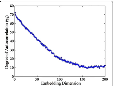
Fig. 2Autocorrelation of the wind speed data
Table 1The forecasting errors based on cross-validation
Polynomial kernel function
Wavelet kernel function
MAPE (%) MSE
1 0 8.0793 0.7848
0.1 0.9 7.1208 0.6269
0.2 0.8 7.0743 0.6238
0.3 0.7 7.0399 0.6208
0.4 0.6 7.0442 0.6203
0.5 0.5 7.0559 0.6208
0.6 0.4 7.0639 0.6208
0.7 0.3 7.0833 0.6218
0.8 0.2 7.0997 0.6229
0.9 0.1 7.1543 0.6291
Eq. (8), and the normalization of the test set sample xi′ is the same as that ofxi.
~xi¼PN xNð i−xÞ i ðxi−xÞ
ð8Þ
Here, x is the average value of each component of the sample,Nis the number of training samples (or test sam-ples), and xi is the normalized data. After normalization by formula (8), the sample component values of the training set and test set are between [0, 1].
3 Experimental modeling and analysis
Taking the wind speed data collected by a wind farm in Ningxia in June 2012 as an example, experimental mod-eling was carried out. The wind speed was sampled every minute, and the speed data for 3 days were collected for our experiment. Therefore, there are 4320 samples in total. In the model construction, 70% of them were randomly selected as training data, 30% as prediction samples, and a cross-validation method was used to achieve the model performance comparison.
In this paper, the mean absolute percentage error (MAPE), mean square error (MSE), and maximum permissible error (MPE) are used as criteria to measure the error of the wind speed prediction results.
MAPE¼ 1
In the formulas, vp is the predicted wind speed, vr is the real wind speed, μ is the average value of the predicted samples, and N is the number of predicted
samples. The MAPE and MSE pay more attention to the overall average performance of the prediction model, while the MPE reflects the error control ability of the prediction model for individuals.
Establishing the model mainly includes four steps: feature selection, combined kernel function selection, extraction of similar data and establishment of the prediction model, and wind speed-power conversion.
3.1 Feature selection
Feature selection, with the purpose of extracting the appropriate features from the raw data, is a key step in determining the performance of the support vector ma-chine model. Since the feature is historical wind speed in this model, it is only necessary to select the number of historical wind speeds. As a time series, wind speed has a strong autocorrelation, so the feature selection is guided by the autocorrelation of wind speed sequences. The input sequence of the support vector machine model is xt= [yt−D, yt−D+ 1, …, yt−1]. Dis called the embedding dimension, which is determined by the de-gree of correlation among the data. The selection ofDis evaluated based on the model complexity and prediction accuracy. The formula for calculating autocorrelation is as follows (12):
In the formula, rk is the degree of autocorrelation, and μy and sy are the mean and standard deviation of the wind speed data, respectively. Figure 2 shows the autocorrelation under different embedding dimensions. The horizontal axis is the embedding dimension, and the vertical axis is the autocorrelation. According to the expected autocorrelation threshold, the corresponding number of features can be obtained. In this paper, the
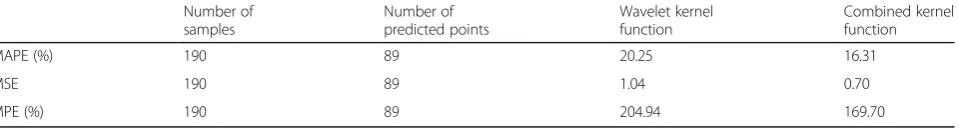
Table 2A comparison of the prediction error between the wavelet kernel function and combined kernel function for 279 samples
Number of
MPE (%) 190 89 204.94 169.70
Table 3A comparison of the prediction error between the wavelet kernel function and combined kernel function for 587 samples
Number of
MSE 411 176 0.66 0.54
autocorrelation threshold is 70%, and the corresponding number of features in the autocorrelation graph is 2.
3.2 Selection of combined kernel functions
The parameter selection of the combined kernel func-tion has two steps. The first step is to determine the parameters of the single wavelet kernel function, and the second step is to determine the combination coefficient of the combined kernel function. According to the com-bination of global and local kernel functions, we first establish a model by using a single wavelet kernel func-tion and a single polynomial kernel funcfunc-tion and find the optimal parameters through the grid method so that the cross-validation prediction obtained by the support vector machine model established by each kernel func-tion is obtained. The error is minimal.
The combined coefficients of the polynomial kernel function and the wavelet kernel function are also deter-mined based on the error results of the cross-check of the training samples. The specific idea is to adjust the respective parameters of the polynomial kernel function and the wavelet kernel function to the optimal state and then set the combination coefficients of different polyno-mial kernel functions and wavelet kernel functions to generate a new combined kernel function, which is ap-plied to the model. The trained model is cross-validated to obtain two error results of MAPE and MSE and then to select the set of combination coefficients with the smallest error. The cross-validation results are shown in Table 1. It can be concluded that when the coefficients of the polynomial kernel function are 0.3 and 0.4 and the coefficients of the wavelet kernel function are 0.7 and 0.6, the MAPE error and MSE error of the model are the smallest. The coefficient combination selected in this paper is 0.4 for the polynomial kernel function and 0.6 for the wavelet kernel function.
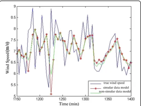
The wind speed data for all days in June are the ori-ginal data, 70% of which are used as training data and 30% as forecast data. As shown in Fig.3, the wind speed prediction results are obtained by combining the kernel function and training the model with a single wavelet kernel function. It can be clearly seen that the wind speed results predicted by the combined kernel function are closer to the real wind speed data. Table 2 gives the error data of the two models. The comparison shows that the model obtained by the combined kernel function
reduces the mean error by 3.94%, the mean square error by 0.34, and the maximum allowable error by 35.24%.
To verify the applicability of the combined kernel function method, we randomly select another 587 wind speed data from the historical wind speed data for a period of time. The data set is completely independent of the above data. The data set is divided into training samples and prediction samples, and the model is built. The wind speed prediction performance is listed in Table3.
3.3 Similar data extraction from training samples
In this paper, when selecting similarity data, the thresh-old ofτis set to 0.5. According to three different trends of wind speed, the models are trained separately. Then, by classifying the trend of changes before the prediction point, the corresponding models are selected to predict this point, and the prediction results are obtained.
The method is applied to a field wind speed prediction experiment of a wind farm in Ningxia. The error results of wind speed prediction are shown in Table4. For intu-ition, the wind speed data from 1150 min to 1400 min in the prediction results are shown in Fig. 4. After adding similar data-classification modeling, the three error indicators have been reduced; that is, the mean error (visible from MAPE and MSE) can be reduced, while the prediction error for a single point can be further reduced (visible from MPE).
Table 4A comparison of the prediction results with and without similar data
Number of samples
Number of predicted points
Combined kernel function
Combined kernel function and similar data
MAPE (%) 882 378 8.64 8.38
MSE 882 378 0.58 0.55
MPE (%) 882 378 41.71 40.23
The results from the field experiments verify the ac-curacy of the system. As the number of on-site samples continues to accumulate, the method will periodically update the training samples and retrain the models to achieve higher prediction accuracy.
3.4 Wind speed-power conversion
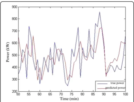
When the predicted wind speed data are obtained, the predicted wind speed can be converted into the pre-dicted power value of a turbine through the correspond-ing relationship between wind speed and power. Wind turbines in wind farms operate mostly in the state of unlimited power. In this state, when the wind speed is constant, the ideal output curve can be obtained theoret-ically. The formula of wind speed-power conversion is shown in formula (13):
In the formula, vcut _ in is the cut-in wind speed,vnorm is the rated wind speed and vcut _ out is the cut-out wind speed. The C(·) function is provided in the manuals of wind turbine suppliers. In this study, the cut-in wind speed of wind turbines is 3 m/s, the cut-out wind speed is 25 m/s, and the rated wind speed is 10.7 m/s.
According to the predicted wind speed data and the wind speed-power conversion formula (13), the pre-dicted power can be obtained, as shown in Fig. 5. This figure shows that the predicted power is very close to the real power and that the tracking ability of the power curve is strong
4 Conclusion
A wind speed prediction experiment based on a certain wind farm in Ningxia shows that the proposed method of combining a kernel function and similar data with a support vector machine can effectively improve the accuracy of wind speed prediction and then improve the accuracy of wind power prediction. The conclusions are as follows:
1) By combining the advantages of different types of kernel functions for wind speed prediction, a higher prediction performance than that of a single kernel function can be obtained.
2) The wind speed historical data are independently modeled and predicted according to the similarity of the changing trend, which can effectively improve the wind speed prediction accuracy.
3) The experimental results of this method at the wind power site show that the method is feasible in engineering applications.
Abbreviations
CFD:Computational fluid dynamics; MAPE: Mean absolute percentage error; MPE: Maximum permissible error; MSE: Mean square error; RBF: Radial basis function; SVM: Support vector machine
Acknowledgements
The wind speed data acquisition and prediction experiment in this paper was completed with the strong support and assistance of some staff members from the Sichuan Dongfang Electric Automatic Control Engineering Co., Ltd. We would like to express our heartfelt thanks to them.
Authors’contributions
JH proposed the main idea, derived the algorithm, and wrote the paper. JX translated the paper into English and revised the paper. All authors read and approved the final manuscript.
Authors’Information
Jian He (1978.5-) is a Lecturer of the University of Electronic Science and Technology of China (UESTC). He obtained a Master’s degree in 2003 from the School of Automation Engineering of the UESTC. He now specializes in artificial intelligence, speech recognition, and radio and television auto-control technology.
Funding
2018JZ0050: Science & Technology Department of Sichuan Province. 2017GZYZF0014: Science & Technology Department of Sichuan Province. 2018SF020: Science and Technology Department of Yibin. 2018ZSF001: Science and Technology Department of Yibin. 2019GY001: Science and Technology Department of Yibin.
Availability of data and materials
Data sharing is not applicable to this article, as no datasets were generated or analyzed during the current study.
Competing interests
The authors declare that they have no competing interests.
Received: 14 January 2019 Accepted: 11 September 2019
References
1. B.C. Ummels, M. Gibescu, W.L.K. EngbertPelgrum, A.J. Brand, Impacts of wind power on thermal generation unit commitment and dispatch [J]. IEEE transactions on energy conversion22(01), 44–51 (2007)
2. Z. Hongyu, Y. Yonghua, S. Hong, et al., Peak-load regulating adequacy evaluation associated with large-scale wind power integration [J]. Proceedings of the CSEE31(22), 26–31 (2011)
3. W. Yaonan, S. Chunshun, L. Xinran, Short-term wind speed simulation corrected with field measured wind speed [J]. Proceedings of the CSEE 28(11), 94–100 (2008)
4. Y. Xiuyuan, XiaoYang, C. Shuyong, Wind speed and generated power forecasting in wind farm [J]. Proceedings of the CSEE11(6), 1–5 (2005) 5. G. Shuang, D. Lei, G. Yang, et al., Mid-long term wind speed prediction
based on rough set theory [J]. Proceedings of the CSEE32(01), 32–37 (2012) 6. Z.-y. Wang, J. Zhi-cheng, Research on grey Verhulst models for
short-term wind speed prediction. Control Engineering of China 20(02), 219–222 (2013) 230
7. P. Huaiwu, L. Fangrui, Y. Xiaofeng, Short term wind speed forecast based on combined prediction [J]. ActaEnergiae Solaris Sinica32(04), 543–547 (2011) 8. C.S. Watters, P. Leahy, Comparison of linear. Kalman filter and neural network
downscaling of wind speeds from numerical weather prediction [C]. International conference on Environment and ElectricalEngineering, 1–4 (2011) 9. P. Difu, L. Hui, Y. Li, A Wind speed forecasting optimization model for wind
farms based on time series analysis and Kalman filter Algorithm [J]. Power System Technology32(07), 82–86 (2008)
10. Liang, L., F. Shao. The study on short-time wind speed prediction based on time-series neural network algorithm [C]. Power and Energy Engineering Conference (APPEEC), 2010 Asia-Pacific,2010,1-5.
11. S. Gao, Y. He, H. Chen, Wind speed forecast for wind farms based on ARMA-ARCH model [C]. International Conference on Sustainable Power Generation and Supply, 1–4 (2009)
12. P. Difu, L. Hui, Y. Li, Optimization algorithm of short-term multi-step wind speed forecast [J]. Proceedings of the CSEE28(26), 87–91 (2008) 13. J. Ignacio, L. Alfredo, M. Claudio, et al., Comparison of two new short-term wind
power forecasting systems [J]. Renewable Energy34(7), 1848–1854 (2009) 14. T.G. Barbounis, J.B. Theocharis, M.C. Alexiadis, et al., Long-term wind speed
and power forecasting using local recurrent neural network models [J]. IEEE Transactions on Energy Conversion21(1), 273–284 (2006)
15. X. Li, Y. Liu, W. Xin, Wind speed prediction based on genetic neural network [J]. Industrial Electronics and Applications (ICIEA), 2448–2451 (2009) 16. D. Lang, H.K. HuangShoudao, et al., Combination forecasting model based
on neural networks for wind speed in wind farm [J]. Proceedings of the CSU-EPSA23(04), 27–31 (2011)
17. F. Shu, J.R. Liao, R. Yokoyama, et al., Forecasting the wind generation using a two-stage network based on meteorological information [J]. IEEE Transactions on Energy Conversion24(2), 474–482 (2009)
18. F. Gaofeng, W. Weisheng, L. Chun, et al., Wind power prediction based on artificial neural network [J]. Proceedings of the CSEE28(34), 118–123 (2008) 19. L. Chun-Yao, H. Yan-Lou, Wind prediction based on general regression
neural network [C]. International Conference onIntelligent System Design and Engineering Application, 617–620 (2012)
20. C. Niya, Q. Zheng, M. Xiaofeng, et al., Multi-step ahead wind speed forecasting model based on spatial correlation and support vector machine [J]. Transactions of China Electrotechnical Society28(05), 15–21 (2013) 21. W. Li, S.G. WeiZhinong, et al., Multi-interval wind speed forecast model
based on improved spatial correlation and RBF neural network [J]. Electric Power Automation Equipment29(06), 89–92 (2009)
22. W. Junli, Z. Buhan, W. Kui, Application of Adaboost-Based BP Neural Network for Short-Term Wind Speed Forecast [J]. Power System Technology 36(09), 221–225 (2012)
23. Y. Xiyun, S. Baojun, Z. Xinfang, et al., Short-term wind speed forecasting based on support vector machine with similar data [J]. Proceedings of the CSEE32(04), 35–41 (2012)
24. P. SangitaB, S.R. Deshmukh, Use of support vector machine for wind speed prediction [C]. International Conference on Power and Energy Systems, 1–8 (2011) 25. Z. Jianwu, Q. Wei, Short-term wind power prediction using a wavelet
support vector machine [J]. IEEE Transactions onSustainable Energy 3(02), 255–264 (2012)
26. Z.B. ZhangGuoqiang, Wind speed and wind turbine output forecast based on combination Method [J]. Automation of Electric Power Systems33(18), 92–95 (2009) 27. A.-n. Wang, Y. Zhao, Y.-t. Hou, et al., A novel construction of SVM
compound kernel function [C]. International Conference onLogistics Systems and Intelligent Management, 1462–1465 (2010)
28. J. Bai, X.-y. Zhang, Y.-l. Guo, Speech recognition based on a compound kernel support vector machine [C]. IEEE International Conference on Communication Technology, 696–699 (2008)
Publisher’s Note