Determination of density contrasts for a three-dimensional
sub-surface intermediate layer
I. L. Ateya1and S. Takemoto2
1Department of Geomatics Engineering and Geo-spatial Information Systems, Jomo Kenyatta University of Agriculture and Technology,
P. O. Box 62000, Nairobi, Kenya
2Department of Geophysics, Kyoto University, Kitashirakawa Oiwake-cho, Sakyo-ku, Kyoto 606-8502, Japan (Received January 9, 2003; Revised August 29, 2003; Accepted August 29, 2003)
The quantitativedetermination of the variable density contrasts for an intermediate horizontal layer has been demonstrated. In particular a sub-surface dipping dike with aprioridepth-dependent density contrasts was adopted as aforward modelto project gravity anomaly effect above the Earth surface. The sub-surface location and density contrasts in a series of intermediate horizontal layers in the causative dipping dike structure have been recovered by means of inversion analysis. Density contrasts recovery errors of less than 8.0 percent were realized to a depth of 2.00 km on a maximum synthetic gravity anomaly effect of 10.0 mGals that is better in comparison to constant density models. Finally to demonstrate the efficacy of the inverse analysis in the study, the entire process was successfully applied to real field data, i.e., residual gravity anomaly for a micro-gravimetry site and/or localized structures in Matsumoto Basin, Chubu District—Japan.
Key words:Density contrasts, intermediate horizontal layer, sub-surface dipping dike.
1.
Introduction
The solution of problems in inverse theory and/or down-ward continuation of potential fields into arbitrary regions of the lower half-space are extensive in geophysical literature. Notably the research works of Savinsky (1963, 1967, 1984, 1995) and Savinskyet al.(1981) among other authors. For example, Savinsky et al. (1981) determines by downward continuation in the lower half-space the disturbing masses in a horizontal layer. Further, the entire lower half-space is similarly considered for disturbing masses for an interme-diate layer from observed potential fields, i.e., gravity and magnetism in Savinsky (1984).
When density varies in the lower half-space or within a sub-surface structure it results in what is referred to as vari-able density. The density contrasts are then the difference between the structure’s density and density of surrounding geological materials assumed to be homogeneous. In seek-ing to explain the gravity anomalies, density variations are considered and these have a direct relationship with the sub-surface structure’s disturbing masses. In order to distinguish the different materials, then density contrasts are sought in the different layers in the lower half-space.
The gravity anomaly of a complicated two-dimensional source having arbitrary surfaces and the density distribution separated by either horizontal or vertical direction can be cal-culated using a combination of a closed form solution or nu-merical interpretations (Ruotoistenmaki, 1992). Rao (1986a, 1990) considered the problem of variable density contrasts and derived the gravity anomalies of prisms and trapezoids having second-degree polynomial density distributions in the
Copy right cThe Society of Geomagnetism and Earth, Planetary and Space Sciences (SGEPSS); The Seismological Society of Japan; The Volcanological Society of Japan; The Geodetic Society of Japan; The Japanese Society for Planetary Sciences.
vertical directions.
Modeling of regular sub-surface structures e.g., dikes and faults, to depict their anomaly patterns in the lower half-space has been tackled extensively in Geldartet al. (1966) and Telford et al.(1990). Other authors have studied two-dimensional gravity models with variable density contrasts, e.g., Cordell (1973), Murthy and Rao (1979), Martin-Atienza and Garcia-Abdeslem (1988). A more general approach is by Guspi (1990) who considered gravity sources bounded by polygons and having polynomial density distribution varying with depth.
Li and Oldenburg (1996, 1998) on the other hand, pro-posed a sub-surface model of a dipping dike with a con-stant density throughout its volume. The gravity anomaly ef-fect was then transformed to pseudo-magnetic anomaly and adopted for the recovery of the locations and/or parameters of the sub-surface structures. The sub-surface locations with respect to depth and the lateral variations were a key interest in Li and Oldenburg (1996, 1998) contributions.
Assuming a uniform or variable contrasts in the sub-surface it is possible to calculate from the potential field signals the probable geometry of the causative structure. Boulanger and Chouteau (2001) adopted a dipping dike model similar to that of Li and Oldenburg (1996, 1998) but introduced the rectangular parameterizations, i.e., den-sity units to the sub-surface structure.
In our case, we adopt a variant of the dipping dike model and introduce a depth-dependent density contrasts factor in the sub-surface structure. Effectively the density contrasts in the structure with respect to depth of horizontal layers are known apriori. We attempt the recovery of the sub-surface density contrasts in the dipping dike at varying depths and intermediate layer heights in three-dimensions.
( )z
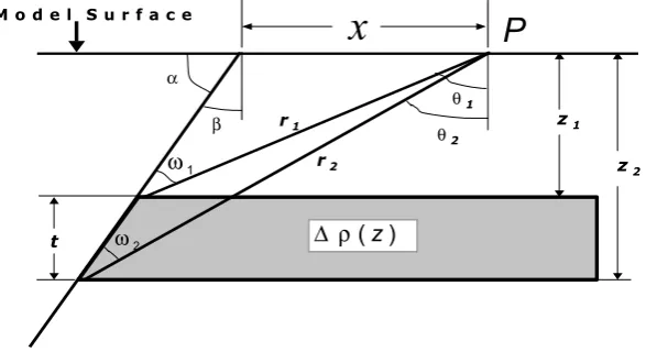
Fig. 1. Parameters and/or variables for gravity anomaly effect of a horizontal slab.
Table 1. Density in the intermediate layers in the dipping dike.
Layer Depth of layer Density contrasts Differences in (km) (g/cm3) contrasts (g/cm3)
Modeling is one of the most important tools in geophys-ical sciences as it allows a quantitative prediction and es-tablishment of relations to measurements of real objects. In order to understand how a model influences particular po-tential field data one must be able to calculate theoretical or synthetic data for an assumed contrived Earth model, which constitutes theforward problem. This sometimes involves deriving a mathematical relationship between the data and the contrived model.
2.1 Location characteristics
Starting from synthetic gravity anomaly effects, which ex-plain density variations in the sub-surface structure, the goal is to recover the structure density contrasts per each horizon-tal layer by invoking a valid model. Assuming a sub-surface structure that consists of nearly homogenous sediments we simulate a regular dipping dike-like structure. The causative structure is such that one face, i.e., namely XZ has dip angle of 45◦, a second YZ face resembles a finite horizontal slab and a top XY face is a regular square. The three faces form a regular three-dimensional dipping dike model (cf. Boulanger and Chouteau (2001)
2.2 Geological materials and density contrasts
Rock densities prominently feature in the analysis of sub-surface structures and therefore in the interpretation of grav-ity anomalies, it is necessary to estimate the densities of the sub-surface rocks before one can postulate their structure. For this reason it is desirable to adopt some geological data
on the densities of the representative rocks in regions where the gravity surveys are made. It should be pointed out that it is not the absolute densities but the density contrasts that are significant. In this study we adopted the geological materials similar to those in Ateya and Takemoto (2002a,b).
The variation in density contrasts with depth can be ap-proximated by a smooth function either quadratic or expo-nential by least squares fitting of the function to the observed data (Rao, 1986a; Zhanget al., 2001). Further Zhanget al. (2001) studied gravity anomalies of two-dimensional bod-ies with layers of variable density contrast like rectangular cylinders and inclined fault models. Following after Rao (1986b) and Zhanget al.(2001) we approximated the depth-dependent variable density contrasts for a sub-surface dip-ping dike based on geological materials in Ateya and Take-moto (2002a,b) as:
ρ(z)= −0.515+0.109z−0.003z2 (1)
Table 1 shows the layer density contrasts and the con-trasts differences between the respective intermediate hor-izontal layers. The density contrast at top surface (depth equal zero) is same as the difference between the average alluvial deposits of density 2.12 g/cm3 and the average
re-duction density of 2.645 g/cm3in the region after Yamamoto
et al.(1982), i.e.,ρ(0)= −0.525.
Most of the geological materials used in the synthetic modeling are from Central Ranges in the Japan Alps and therefore the reduction density adopted was 2.645 g/cm3, a
value closer the average value of 2.64 g/cm3 by Yamamoto
et al.(1982).
The value was obtained by a least squares method that incorporates the topography that covers an extensive 40,000 km2 with elevation heights ranging from 0 to 3000 m for which the Earth’s sphericity cannot be ignored (Yamamoto et al., 1982).
i
θ
β
b
Fig. 2. Parameters and/or variables describing the gravity anomaly effect of a sub-surface dike-like structure.
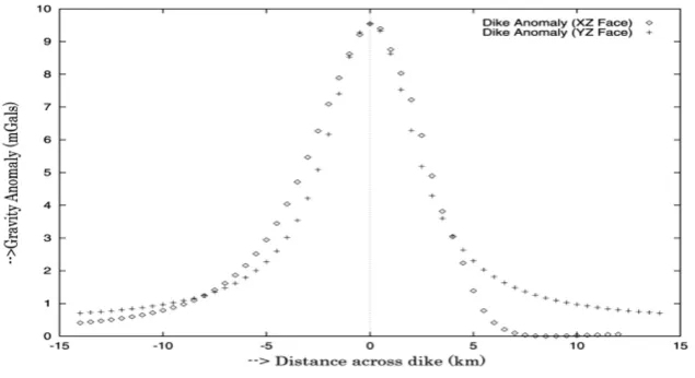
Fig. 3. Gravity anomaly effects of the independentX ZandY Zdike faces with point-to-point spacing 0.50 km.
2.3 Gravity anomaly
For simplicity we assume synthetic data interpolated onto a regular rectangular grid over the sub-surface dipping dike. The top surface of model is assumed to coincide with a flat Earth surface. Independently theY Z face is modeled as fi-nite sub-surface horizontal slab with the different parameters are shown in Fig. 1 wherexis the distance of an observation point P,t is the thickness of slab,β is the complement of the dip angleα, whilez1andz2are the depths to the top and
bottom of the slab respectively.
Further, in Eq. (2)G is the gravitational constant while ρ(z)are variable density contrasts. The depth to top sur-face, i.e., model Earth surface z1 is 0.025 km, depth to the
bottomz2is 4.050 km and widths of 3.050 km in the
regu-larxandydirections. The gravity anomaly effectgobs, of a
two-dimensional finite horizontal slab is given by Geldartet al.(1966) and Telfordet al.(1990) as in Eq. (2).
gobs=2Gρ(z)
πt 2
+(z2θ2−z1θ1)+x(θ2−θ1)
·sinβcosβ+xcos2βln
r2
r1
(2)
The X Z face can be modeled as a sub-surface dike-like
structure with its different parameters depicted as in Fig. 2. The distance x is positive when the point P is to the right of central position with all angles being measured in the clockwise direction. The anglesβandθiare measured from the vertical and α from the plane with zi as the depth in the sub-surface. A two-dimensional dike can be obtained by the subtraction of two slabs one being displaced horizontally with respect to the other. The gravity anomaly effectgobsof
such a dike-like structure is given by Geldartet al. (1966) and Telfordet al.(1990) as Eq. (3):
gobs=2Gρ(z) z2 (θ2−θ4)−z1(θ1−θ3)+sinβcosβ · {x(θ2+θ3−θ4−θ1)+b(θ4−θ3)} + cos2β
xln
r2r3
r1r4
+bln
r4
r3
(3)
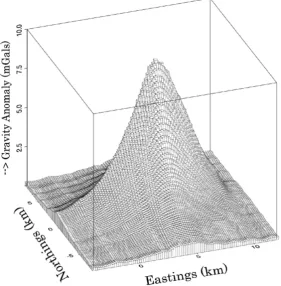
Fig. 4. Synthetic gravity anomaly effect of the three-dimensional sub-surface dipping dike displaced eastwards by 5.0 km.
anomaly effect of the two faces was 9.50 mGals as shown in Fig. 3.
The gravity anomaly effects of the two-dimensional inde-pendent faces were generated to cover the entire rectangular grid and superimposed onto each other with each co-ordinate having a gravity anomaly effect from each face interpolated directly above the grid nodes to form one overall system of gravity anomaly effects.
The resultant gravity anomaly effect was then further modeled and analyzed dependent on the co-ordinate lo-cations to have a maximum anomaly equal to the maxi-mum gravity anomaly effect of each independent face. The data was then contaminated by un-correlated Gaussian noise of maximum amplitude of 0.50 mGals. The final gravity anomaly effect was deliberately shifted by 5.00 km East-wards to enable investigate for apparent shifts in the sub-surface structure. The peak gravity anomaly effect was main-tained at 9.50 mGals. The resultant three-dimensional syn-thetic gravity anomaly effect for the sub-surface dipping dike-like structure is shown in Fig. 4.
3.
Inversion Analysis
Solving an inverse problem means making inferences about physical systems from observation data. The grav-ity inverse problem is an ill-posed problem in the sense of Hadamard (1902) because its solution is neither unique nor stable. The non-uniqueness of the inverse problem increases rapidly for bodies with in-homogenous density and rapidly becomes unmanageable. The stable solution is possible thanks to regularization techniques on the basis of the gen-eral principles enunciated by Tikhonov and Arsenin (1974)
and/or Tikhonov and Glasko (1965).
The disturbing or gravitating masses in the lower half-space (z>0) can be reflected in the potential field observed on the Earth’s surface. The problem of finding the different densities in the entire lower half-space belowh = H0was
previously considered in Savinsky (1984) where the limit for was at infinity instead of H0+H. For similar cases the
problem is to derive the greatest possible amount of infor-mation on the positions, locations and the sub-surface struc-tures of the causative sources from the measurements of po-tential fields, e.g., the field observed gravitational anomalies, g(xj,yj,zj).
A possible sub-surface location in the horizontal layer can be at a depth from h = H0 to h = H0 +H, where
H the thickness of the horizontal layer andQ(x,y,h)the disturbing masses that represent the density distributions. If one assumes that there are values of the potential field g(xj,yj,zj), j = 1,2. . .N, where zj are deviations in the vertical direction from the horizontal measurements level h = 0, then the solution of the problem can be achieved through Eq. (4):
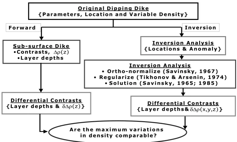
polyno-Fig. 5. Quantitative determination of the density contrasts in an intermediate horizontal layer.
Table 2. Differences between aprioriand inversion analysis density contrasts.
Depth of layer Model density Inversion analysis Differences (km) contrasts (g/cm3) contrasts (g/cm3) (g/cm3)
0.000 0.000 0.000 0.000
0.400 0.032 0.028 0.004
0.800 0.042 0.045 −0.003
1.200 0.042 0.038 0.004
1.600 0.041 0.046 −0.005
2.000 0.039 0.054 −0.015
Table 3. Location of investigation site in Chubu District.
Longitude Latitude Height above Residual anomaly
(Deg.) (Deg.) sea level (m) (mGals)
Minimum 137.875 36.320 500.342 −5.425
Maximum 137.975 36.420 702.808 8.175
Difference 0.100 0.100 202.466 13.600
mial form, the terms of which are formed by the functions of the kernel of the integral equation (Savinsky, 1963; Savinsky et al., 1981). The resulting density distribution or disturbing masses Q(x,y,h)in Eq. (4) have a physical meaning only atH0<h < H0+Hand therefore a series of horizontal
layers taken to cover the entire lower half-space.
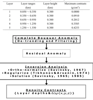
Figure 5 shows the flow diagram that incorporates sub-surface model; the procedure of the inversion analysis for the determination of the variable density contrasts in a series of intermediate horizontal layers. The differences between the differential density contrasts from forward modeling and inversion analysis for each horizontal layer are given in Ta-ble 2.
Table 2 shows the inversion analysis contrasts where the heights of the horizontal layers are kept constant atH = 0.400 km although several different horizontal layer heights
were actually investigated. The second column represents the differential density contrasts from the forward model ρ(z)using a reduction density of 2.645 g/cm3 given that
ρ(0) = −0.525 while the third column represents the maximal density contrasts ρ(x,y,z) in each respective horizontal layer. Fourth column shows the differences be-tween the aprioriand recovery density contrasts. Figure 6 shows density contrasts for an intermediate horizontal layer of depth range 0.400∼0.800 km with a contour interval of 0.003 g/cm3.
4.
Application with Actual Field Data
Fig. 6. Density contrasts for an intermediate horizontal layer of depth range 0.400∼0.800 km with a contour interval of 0.003 g/cm3.
1 0.050∼0.350 0.300 0.0800
2 0.350∼0.650 0.300 0.0910
3 0.650∼0.950 0.300 0.2012
4 0.950∼1.250 0.300 0.3585
5 1.250∼1.550 0.300 0.4253
Fig. 8. Determination of the density contrasts in a horizontal layer using residual anomaly.
complete Bouguer anomaly of the region was computed with the adopted average topographic density as 2.64 g/cm3after of Yamamotoet al.(1982).
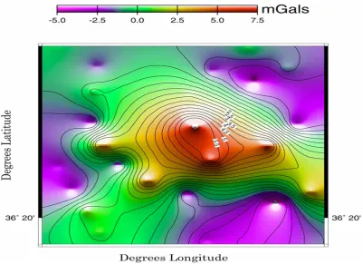
A major step in the analysis of the gravity data is the pro-cess of isolating the observed anomaly patterns into regional and residual components (Chapin, 1996). The complete Bouguer anomaly of the encompassing region was computed and the residual anomaly determined for the investigation site given in Table 3 using data obtained from Geological Survey of Japan (2000). Figure 7 gives the residual anomaly of the investigation site that was utilized.
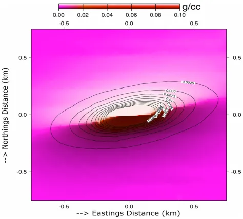
In both de-trending and filtering we utilized the GMT soft-ware prepared by Wessel and Smith (1995). The compu-tation of the density contrasts in a series of horizontal lay-ers with different heights in the sub-surface proceeds as in Fig. 8. It helps determine the depth-dependent density con-trasts ρ(x,y,z) from the residual anomaly by inversion analysis. The point-to-point separation was maintained at 0.50 km in the final interpolated values on the grid. The in-version analysis results for the density contrasts for a sub-surface horizontal layer of range 0.350 ∼ 0.650 km are shown in Fig. 9.
Similar inversion analysis results for a series of horizon-tal layers of same thickness, i.e., each with a layer height of 0.300 km was performed and the summary is given in Ta-ble 4. The inversion analysis was performed to a depth of 1.60 km. The contour of the disturbing masses gives a pos-sible density contrasts in the structure at the location.
Table 4 shows the maximum density contrasts for a pos-sible density contrasts structure in Matsumoto basin, Chubu District. The density or density contrasts of the sub-surface could then be obtained by relating the density or density con-trasts to the Earth surface between the subsequent intermedi-ate horizontal layers.
5.
Discussion and Conclusions
It has been shown that it is possible to determine or recover the intermediate layer density contrastsρ(x,y,h)changes with respect to depth from inversion analysis. The error differences are less than 5.0 mg/cm3 up to a depth of 2.00
km for the horizontal layers of 0.400 km thickness have been realized.
In this case the depth-dependent density contrasts forward modelρ(z)was computed apriorifor a series of interme-diate horizontal layers with varying heights and at different depths. The same heights were utilized in the inversion anal-ysis to determine if it is possible to recover the maximum values i.e., quantities in the forward model.
The differences increase gradually after a depth of 2.00 km in the sub-surface. One possibility for the increase is due to use of greater point-to-point separation distance with in-creasing depth. It effectively smoothens the effective gravity anomaly effect as noted in Savinsky (1967), i.e., set of in-version results become poorly defined at increasing depths H0 due the influence of the accumulated errors or
point-Fig. 9. Density contrasts results for a horizontal layer of range 0.350∼0.650 km with a contour interval of 0.0025 g/cm3.
to-point separations. These accumulated errors calls for the need for regularization techniques applied in the inversion analysis (Tikhonov and Arsenin, 1974; Koch, 1990).
We chose the maximum values (quantities) per interme-diate layer because of the maximum gravity anomaly effect maintained at either central or shifted locations. Each max-imum value mirrors the highest value of density contrasts for each intermediate layer possible from the synthetic dip-ping dike model. Similar inversion analysis was applied to an investigation site for a real field data in Matsumoto basin, Chubu District.
Results of the investigation site for a possible sub-surface structure in Matsumoto basin, Chubu District are depicted in fourth column of Table 4 with maximum density contrasts for a series of intermediate horizontal layers. In conclusion in the present study, the determination of a priori depth-dependent density contrasts within an intermediate horizon-tal layer has been quantitatively demonstrated. Closely re-lated to the disturbing masses in an intermediate horizontal layer the recovery of density contrasts in the actual location of the causative structure in the sub-surface has been
demon-strated too. The determination of disturbing masses is more effective in micro-gravimetry studies and/or localized struc-tures without the effects of long-wavelength potential field anomalies and a more accurate interpretation is dependent on the abundance of geological information.
Acknowledgments. We would like to express our gratitude to Ge-ological Society of Japan (GSJ) for the entire gravity data and part of the geological data utilized in this research as provided on the Gravity CD-ROM for Japan dated 24th March 2000. Further our thanks to Geographical Survey Institute (GSI) for the Digital Ter-rain Data for the Japan Alps region and the extra gravity data espe-cially in Matsumoto Basin.
References
Ateya, I. L. and S. Takemoto, Inversion of gravity across a sub-surface dike-like structure in two dimensions. Western Pacific Geophysics Meet-ing (WPGM), WellMeet-ington, New Zealand,EOS Trans. AGU,83(22), 112, 2002a.
Ateya, I. L. and S. Takemoto, Gravity inversion modeling across a 2-D dike-like structure—A Case Study,Earth Planets Space,54, 791–796, 2002b. Boulanger, O. and M. Chouteau, Constraints in 3-D gravity inversion,
Geo-physical Prospecting,49, 265–280, 2001.
dimensional faults,Geophysics,31(2), 372–397, 1966.
Geological Survey of Japan (GSJ), Gravity CD-ROM of Japan published on 24th March 2000, URLhttp://www.gsj.go.jp.
Guspi, F., General 2-D gravity inversion with density contrasts varying with depth,Geo-exploration,26, 253–265, 1990.
Hadamard, J., Sur les problemes aux derive espartielles et leur signification physique, Bulletin of Princeton University,13, 1–20, 1902.
Koch, M., Optimal regularization of the linear seismic inverse problem, Technical Report No. FSU-SCRI-90C-32, Florida State University, Tal-lahassee, Florida, 1990.
Li, Y. and D. W. Oldenburg, 3-D inversion of magnetic data,Geophysics, 61, 394–408, 1996.
Li, Y. and D. W. Oldenburg, 3-D inversion of gravity data,Geophysics, 63(1), 109–119, 1998.
Martin-Atienza, B. and J. Garcia-Abdeslem, 2-D gravity modeling with an-alytically defined geometry and quadratic polynomial density functions,
Geophysics,64, 1730–1734, 1988.
Murthy, I. V. R. and D. B. Rao, Gravity anomalies of two-dimensional bodies of irregular cross-section with density contrast varying with depth,
Geophysics,44, 1525–1530, 1979.
Rao, D. B., Analysis of gravity anomalies over an inclined fault with quadratic density function,Pageoph,123, 250–260, 1986a.
Rao, D. B., Modeling of sedimentary basins from gravity anomalies with variable density contrast,Geophysics Journal of the Royal Australian Society,84, 207–212, 1986b.
Rao, D. B., Analysis of gravity anomalies of sedimentary basins by asym-metrical trapezoidal model with quadratic function,Geophysics,55, 226– 231, 1990.
Ruotoistenmaki, T., The gravity anomaly of two-dimensional sources with
Ser. Geofiz, No. 5, 712–721, 1963.
Savinsky, I. D., On solving incorrect problems of recalculation of the po-tential field to underlying levels, Izvestiya Academy of Sciences, USSR Physics of Solid Earth, No. 6, 72–92, 1967.
Savinsky, I. D., Solving inverse problems on gravity data with help of kern functions of integral equations, inApplied Geophysics,109, pp. 86–95, Nedra, Moscow, 1984.
Savinsky, I. D., On determination of the contact interface from gravitational and magnetic field, Physics of the Solid Earth, English Translation, 30, No. 10, pp. 903–907, 1995.
Savinsky, I. D., V. L. Briskin, and A. A. Petrova, Reduction of the Grav-itational and Magnetic inclined and Vertical Planes in the Lower Half-Space,Izvestiya Earth Physics,17(12), 934–943, 1981.
Telford, W. M., L. P. Geldart, and R. E. Sheriff,Applied Geophysics,2nd Edition, Cambridge University Press, New York, 1990.
Tikhonov, A. N. and A. Y. Arsenin,Methods of Solving Incorrectly Posed Problems,Nauka, 224, Moscow, 1974.
Tikhonov, A. N. and V. B. Glasko, Application of the regularization method in nonlinear problems, J. Comp. Math. Math. Phys,5(3), 363–373, 1965. Wessel, P and W. H. F. Smith,The Generic Mapping Tools (GMT) Version
3.0 Technical Reference and Cookbook,SOEST/NOAA, 1995. Yamamoto, A., K. Nozaki, Y. Fukao, M. Furumoto, R. Shichi, and T. Ezaka,
Gravity survey in the Central Ranges, Honshu, Japan,Journal of Physics of the Earth,30, 201–243, 1982.
Zhang, J., B. Zhong, X. Zhou, and Y. Dai, Gravity anomalies of 2-D bodies with variable density contrast,Geophysics,66(3), 809–813, 2001.