Neural Network Based Smart Sensor Framework Operating in a Harsh Environment

(1)

Neural-Network-Based Smart Sensor Framework

Operating in a Harsh Environment

Jagdish C. Patra

Division of Computer Communications, School of Computer Engineering, Nanyang Technological University, Singapore 639798

Email:[email protected]

Ee Luang Ang

Narendra S. Chaudhari

Division of Information Systems, School of Computer Engineering, Nanyang Technological University, Singapore 639798

Amitabha Das

Received 11 February 2004; Revised 5 July 2004; Recommended for Publication by John Sorensen

We present an artificial neural-network- (NN-) based smart interface framework for sensors operating in harsh environments. The NN-based sensor can automatically compensate for the nonlinear response characteristics and its nonlinear dependency on the environmental parameters, with high accuracy. To show the potential of the proposed NN-based framework, we provide results of a smart capacitive pressure sensor (CPS) operating in a wide temperature range of 0 to 250◦C. Through simulated experiments, we have shown that the NN-based CPS model is capable of providing pressure readout with a maximum full-scale (FS) error of only±1.0% over this temperature range. A novel scheme for estimating the ambient temperature from the sensor characteristics itself is proposed. For this purpose, a second NN is utilized to estimate the ambient temperature accurately from the knowledge of the oﬀset capacitance of the CPS. A microcontroller-unit- (MCU-) based implementation scheme is also provided.

Keywords and phrases:intelligent sensors, artificial neural networks, autocompensation.

1. INTRODUCTION

In many practical application areas of avionics, automobiles, robotics, missile guidance, oil drilling, and industrial mea-surements, sensors operate in harsh environments such as extreme ambient temperature, pressure, humidity, and so forth. In such situations, the response of the sensors de-pends not only on the measurand but also on the environ-mental parameters in a nonlinear manner. Usually, an exact mathematical model of a sensor showing the relationship be-tween the measurand and its response, and its dependency on the environmental parameters, is not available. Further, since most of the sensors exhibit some amount of nonlinear response characteristics, and the environmental parameters influence the sensor behavior nonlinearly, the problem of ob-taining an accurate readout and its calibration becomes more complex.

(2)

Recently, artificial neural networks (NNs) have emerged as a powerful learning technique to perform complex tasks in dynamic environments. These networks are endowed with certain unique characteristics such as the capability of uni-versal approximation, generalization, and fault tolerance. Be-cause of these characteristics, there have been numerous suc-cessful applications of NNs in various fields of science, en-gineering, and industry [8,9, 10]. It has been shown that the NN-based approximations to measurement data perform better than those of the classical methods of data interpo-lation and least mean square regression [11]. Application of NNs with superior performance for several instrumen-tation and measurement applications have been reported [12,13,14,15,16,17,18].

The main objective of this paper is to demonstrate the potential of NNs in the development of smart sensors ca-pable of mitigating adverse eﬀects of environmental param-eters on the response characteristics of any type of sensor. For this purpose, we propose a multilayer perceptron (MLP)-based scheme to provide linear response characteristics with accurate pressure readout, and to compensate for the non-linear temperature dependency of a capacitive pressure sen-sor (CPS) operating in a harsh environment with tempera-ture variations from 0 to 250◦C. We have assumed that the temperature influences the sensors’s response characteris-tics nonlinearly and have performed simulation studies with three types of nonlinear dependencies.

An inverse model of the CPS is obtained by training a small-sized MLP using the popular backpropagation (BP) learning algorithm [8]. A small-sized MLP is preferable as the training time, computational complexity, and memory requirements decrease with the size of the MLP. To obtain ambient temperature information, a separate temperature sensor is usually embedded with the pressure sensor. An important contribution of this paper is that we have pro-posed a novel scheme to estimate the ambient temperature from the sensor characteristics itself, using a second MLP, thus eliminating the need of a separate temperature sensor. The performance of the NN-based scheme is compared with a polynomial-based interpolation scheme, and it is shown that the NN-based scheme outperforms the interpolation scheme.

The rest of the paper is arranged as follows. Section 2 presents a brief theoretical background of the CPS and the switched-capacitor interface (SCI).Section 3provides details of the proposed MLP-based sensor modeling scheme. The simulated experiments are detailed in Section 4. Section 5 provides performance evaluation and discussions on results of these experiments. The performance comparison with a polynomial-based interpolation scheme is presented in Section 6. A microcontroller-unit-(MCU-) based implemen-tation scheme is provided inSection 7, and finally, conclu-sions of the present study are drawn inSection 8.

2. CPS AND SCI

A CPS senses the applied pressure in the form of elastic de-flection of its diaphragm. The capacitance of a CPS resulting

from the applied pressurePat the ambient temperatureTis given by

C(P,T)=C0(T) +∆C(P,T), (1)

where ∆C(P,T) is the change in capacitance andC0(T) is

the oﬀset capacitance, that is, the zero-pressure capacitance, both at the ambient temperature T. The above capacitance may be expressed in terms of capacitances at the reference temperatureT0as

C(P,T)=C0f1(T) +∆C

in capacitance, both at the reference temperature T0. The

nonlinear functions f1(T) and f2(T) determine the eﬀect of

the ambient temperature on the sensor characteristics [3]. This model provides suﬃcient accuracy in determining the influence of temperature on the sensor’s response character-istics.

When pressure is applied to the CPS, its change in capac-itance at the reference temperatureT0is given by

∆CP,T0

=C0PN 1−τ

1−PN, (3)

whereτis the desensitivity parameter,PN is the normalized applied pressure given byPN =P/Pmax, andPmaxis the

max-imum permissible applied pressure. The parameters τ and Pmax depend on the geometrical structure and physical

di-mensions of the CPS.

In this study, in conformance with practical conditions, we have considered that the ambient temperature influences the CPS characteristics nonlinearly. The nonlinear functions involved are given by

fi(T)=1 +gi(T), (4) gi(T)=κi1Tn+κi2Tn2+κi3Tn3, (5) where Tn = (T−T0)/Tmax. The coeﬃcientsκij,i = 1, 2,

j=1, 2, 3, determine the extent of nonlinear influence of the temperature on the sensor characteristics. Note that when κij = 0 for j = 2 and 3, the influence of the temperature on the CPS response characteristics is linear. The maximum permissible temperature at which the sensor may be oper-ated is denoted byTmax. Let the normalized temperatureTN be given byTN = T/Tmax. The normalized capacitanceCN

may be expressed as

(3)

θ

Figure1: The switched-capacitor interface circuit.

pressure is zero, thenγbecomes zero. Therefore, the normal-ized zero-pressure capacitance, that is, the normalnormal-ized oﬀset capacitance is given by

CN0=f1(T)=1 +g1(T). (8)

SCI for the CPS is shown inFigure 1, where the CPS is represented byC(P). The SCI output provides a voltage sig-nal proportiosig-nal to the capacitance change in the CPS due to the applied pressure. The SCI operation can be controled by a reset signalθ. When ¯θ = 1 (logic 1),C(P) charges to the reference voltageVRwhile the capacitorCSis discharged to ground. On the other hand, whenθ=1, the total charge C(P)VRstored inC(P) is transferred toCSproducing an out-put voltage given by

VO=K·C(P), (9)

whereK =VR/CS. By choosing proper values ofCSandVR, the normalized SCI output VN may be obtained in such a way that

VN =CN. (10)

The unnormalized and normalized SCI outputs at zero-applied pressure are denoted by V00 andVN0, respectively.

Therefore, ifPN =0, thenVN0=CN0.

3. THE MLP-BASED CPS MODEL

We propose an NN-based technique to obtain an inverse model of a CPS to provide accurate pressure readout un-der the nonlinear influence of the ambient temperature. The proposed scheme of the NN-based CPS model for the estima-tion of the applied pressure is shown inFigure 2. This scheme is analogous to the channel equalization scheme used in a digital communication receiver to cancel the adverse eﬀects of the channel on the data being transmitted [8]. To obtain an accurate digital readout of the applied pressure, an MLP-based inverse model of the CPS is used to compensate for the adverse eﬀects of the nonlinear characteristics and its varia-tions due to the influence of the ambient temperature.

In this NN-based CPS model, all the signals used for training and testing are scaled by appropriate SFs to keep their range between 0 and 1. The model operates in two

SF Desired pressure + +

Figure2: The scheme of NN-based modeling of a CPS. (a) Training phase: pressure. (b) Training phase: temperature. (c) Test phase: the complete model.

phases: thetraining phaseand thetest phase. In thetraining phase, the NNs used in the model are trained to learn the sen-sor characteristics and the environmental dependency. The pressure-NN (P-NN) is used to learn the sensor’s response characteristics and its nonlinear dependency on the ambient temperature, whereas the temperature-NN (T-NN) is used to learn the nonlinear function representing variations in the ambient temperature.

We have used MLPs for both the P-NN and the T-NN. Several datasets are needed to train the NNs. An input pat-tern and its corresponding desired, or target patpat-tern consti-tute one pair of data in the dataset. The available datasets are segregated into two parts. The first part, calledtraining set, is used for training of the NNs, and the other part, calledtest set, is used to verify the eﬀectiveness of the model.

3.1. Training phase: pressure

(4)

are generated. The P-NN is trained by taking the patterns from the training set, and its weights are updated by using the popular BP algorithm [8]. After training, the weights of the NN are frozen and stored in an electrically erasable pro-grammable read-only memory (EEPROM). In what follows, the final weights are denoted byWP.

3.2. Training phase: temperature

A scheme to estimate the ambient temperature, by using an-other MLP (T-NN), only from the knowledge of the sensor characteristics is shown in Figure 2b. From (8), it may be seen thatCN0 contains temperature information. However,

since the influence of the temperature on the CPS charac-teristics is considered to be nonlinear, the temperature infor-mation cannot be obtained correctly from the knowledge of CN0, using (8). The T-NN is trained by inputting the values

of VN0 (the normalized SCI output corresponding toCN0,

that is, the SCI output at zero-applied pressure). The desired output is the normalized temperatureTN. Using the BP algo-rithm, the weights of the T-NN are updated. After the train-ing is completed, the final weights are stored in an EEPROM. In what follows, the final weights are denoted byWT.

3.3. Test phase: complete model

The complete scheme of the MLP-based model is shown in Figure 2c. In spite of the variation of the environmental tem-perature and its nonlinear influence on the CPS characteris-tics, this model can estimate the applied pressure accurately. During thetest phaseand actual use of the sensor, the weights WPandWT, stored in the EEPROM, are loaded into the P-NN and T-P-NN, respectively. The P-P-NN has learned the in-verse characteristics of the CPS at diﬀerent values of tem-perature, while the T-NN has learned the nonlinear func-tion representing variafunc-tions of the ambient temperature. The temperature information needed for the P-NN is obtained from the T-NN. The T-NN gets its input from the value of VN0. Next, the input patterns from the test set are applied,

and the model output (PN) is computed. If the model output matches closely with the actual applied pressure (PN), then it may be said that the NN has learned the CPS characteristics correctly. Thereafter, the model can be used along with the CPS to estimate the pressure and to obtain its readout.

4. SIMULATION STUDIES

We carried out extensive simulation studies to evaluate per-formance of the proposed NN-based CPS model. In the fol-lowing, we describe the details of the simulated experiments.

4.1. Preparation of datasets

All parameters of the CPS, such as, ambient temperature, applied pressure, and the SCI output voltage, used in the simulation study were suitably normalized to keep their val-ues between 0 and 1. The datasets needed for training and testing of the NN were generated as follows. The SCI out-put voltage (VN) was recorded at the reference tempera-ture (25◦C) at diﬀerent known values of normalized pres-sure (PN) chosen between 0.0 and 0.6 at an interval of 0.05.

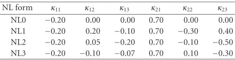
Table1: The values ofκijfor linear and nonlinear forms of

temper-ature dependencies.

NL form κ11 κ12 κ13 κ21 κ22 κ23

NL0 −0.20 0.00 0.00 0.70 0.00 0.00 NL1 −0.20 0.20 −0.10 0.70 −0.30 0.40 NL2 −0.20 0.05 −0.20 0.70 −0.10 −0.50 NL3 −0.20 −0.10 −0.07 0.70 0.10 −0.30

Thus, these 13 pairs of data (PN versusVN) constitute one dataset at the reference temperature. To study the influence of temperature on the CPS characteristics, we have consid-ered three forms of nonlinear functions denoted by NL1, NL2, and NL3, and a linear form denoted by NL0. These were simulated by choosing proper values ofκijin (5). The corre-sponding values ofκijare provided inTable 1.

Next, with the knowledge of the dataset at the reference temperature, and the chosen values ofκij, the response char-acteristics of the CPS for a specific ambient temperature were generated using (7). The response characteristics consist of 13 pairs of data (PN versusVN), and correspond to a dataset at that temperature. For a temperature range from 0◦C to 250◦C, at an increment of 10◦C, twenty-six such datasets, each containing 13 data pairs, were generated. Next, these datasets were divided into two groups: the training set and the test set. The training set, used for training the NNs, con-sists of only five datasets corresponding to 0, 60, 120, 180, and 240◦C, and the remaining twenty one datasets were used as the test set. Let the number of the datasets used for train-ing and the number of data points in a dataset be denoted by NtrgsetandNdatpts, respectively. In the following experiments,

Ntrgset = 5 andNdatpts = 13, and thus, the total number of

training data points is 65 (13×5).

The response characteristics of the CPS for diﬀerent val-ues of temperature (0, 25, 80, 150, and 250◦C) are shown in Figure 3. It may be observed that wide variation in the sensor characteristics occurs when the ambient temperature changes from 0◦C to 250◦C. Further, the sensor’s response characteristics change diﬀerently for the linear form (NL0) and the three nonlinear forms (NL1–NL3) of temperature dependencies.

4.2. Training and testing of the P-NN

A 2-layer MLP with{2−4−1}architecture was chosen in this modeling problem (seeFigure 2a). Initially, all the weights of the P-NN were set to some random values within±1.0. Dur-ing trainDur-ing, a dataset was randomly selected from the five datasets, and a pattern from the selected dataset was also se-lected randomly. The initial values of the learning parameter αand the momentum factorβof the BP algorithm were cho-sen as 0.3 and 0.5, respectively. The MLP architecture and the values ofαandβwere selected after several experiments to provide optimum results.

(5)

0

Figure3: The response characteristics of the CPS operating at diﬀerent temperatures (0, 25, 80, 150, and 250◦_{C) with linear and three forms}

of nonlinear dependencies. (a) NL0. (b) NL1. (c) NL2. (d) NL3.

parameter was used in the BP algorithm. The learning pa-rameter was varied as

αni=αni−1

where ni is the current iteration number, and NITR is the total number of iterations used (in this case, NITR = 100 000). Using a Pentium 4, 2.8 GHz machine, it took only 13 seconds to train the MLP with 100 000 iterations. Finally, the weights of the P-NN (WP) were stored for later use. This procedure was repeated for the linear (NL0) and the three nonlinear forms of temperature influences (NL1–NL3).

The four sets of the final weights (WP) of the P-NN model are provided inTable 2.

(6)

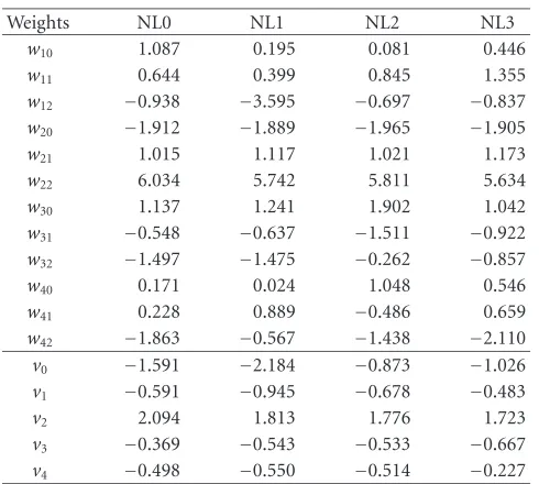
Table2: Final weights (WP) of the P-NN ({2−4−1}architecture).

First layer:wij,i=1, 2, 3, 4, andj =0, 1, 2. Second layer:vk,k =

0, 1,. . ., 4.

Weights NL0 NL1 NL2 NL3

w10 1.087 0.195 0.081 0.446

w11 0.644 0.399 0.845 1.355

w12 −0.938 −3.595 −0.697 −0.837

w20 −1.912 −1.889 −1.965 −1.905

w21 1.015 1.117 1.021 1.173

w22 6.034 5.742 5.811 5.634

w30 1.137 1.241 1.902 1.042

w31 −0.548 −0.637 −1.511 −0.922

w32 −1.497 −1.475 −0.262 −0.857

w40 0.171 0.024 1.048 0.546

w41 0.228 0.889 −0.486 0.659

w42 −1.863 −0.567 −1.438 −2.110

v0 −1.591 −2.184 −0.873 −1.026

v1 −0.591 −0.945 −0.678 −0.483

v2 2.094 1.813 1.776 1.723

v3 −0.369 −0.543 −0.533 −0.667

v4 −0.498 −0.550 −0.514 −0.227

NL0 NL1

NL2 NL3

0 50 100 150 200 250

Temperature (◦C) 0.34

Figure4: Variation of normalized oﬀset capacitance (CN0) of the

pressure sensor with temperature for diﬀerent forms of temperature dependencies.

computed and then compared with the true value of the ap-plied pressure (PN).

4.3. Training and testing of the T-NN

The T-NN was used to estimate the ambient temperature from the knowledge ofCN0at diﬀerent temperatures. For the

chosen values ofκij (seeTable 1), the variation ofCN0 with

the change in temperature for the linear (NL0) and the three forms of nonlinear dependencies (NL1–NL3) are shown in Figure 4. The T-NN was employed to learn these nonlinear functions for estimating the ambient temperature.

Table3: Final weights (WT) of the T-NN ({1−4−1}architecture).

First layer:wij,i = 1, 2, 3, 4, and j = 0 and 1. Second layer:vk,

k=0, 1,. . ., 4.

Weights NL0 NL1 NL2 NL3

w10 −2.277 0.347 −1.328 −0.439

w11 4.070 −0.712 2.765 0.905

w20 2.850 −12.661 0.048 −0.745

w21 −4.611 30.122 −0.099 1.535

w30 −3.558 −6.627 −1.594 −1.891

w31 5.640 12.023 5.446 7.200

w40 −4.577 −5.397 −4.005 −4.997

w41 13.670 11.686 7.333 8.423

v0 2.193 4.525 0.647 0.672

v1 −0.137 0.004 −0.248 −0.021

v2 0.490 −5.263 0.010 −0.027

v3 −1.208 −0.952 −1.041 −1.607

v4 −3.213 0.517 −0.911 −1.403

An MLP with{1−4−1}architecture was chosen for this purpose. During training, the values of VN0 corresponding

to 0, 60, 120, 180, and 250◦C were chosen as the training set (the same temperature values were also used for training the P-NN). The input and desired output of the T-NN were the values ofVN0andTN, respectively (seeFigure 2b).

The initial values of bothαandβwere chosen as 0.7. The updating of the weights was carried out using the BP algo-rithm with a variable learning parameter over 200 000 iter-ations. Using a Pentium 4, 2.8 GHz machine, it took only 2 seconds to train the MLP with 200 000 iterations. The four sets of the final weights (WT) corresponding to the linear and the three nonlinear forms of interaction are tabulated inTable 3.

Testing of the T-NN was carried out after loading the stored weights into the network. The VN0 was varied from

0.35 to 0.55 with an increment of 0.001 and then fed to the MLP. The output of the T-NN and the true value of the nor-malized temperature were compared to verify eﬀectiveness of the model.

5. RESULTS AND DISCUSSIONS

Here, we provide the performance results of the simulation study for the estimation of the applied pressure and the am-bient temperature.

5.1. Estimation of pressure

(7)

0

Figure5: True response characteristics and the pressure estimated by the P-NN model of the CPS operating at diﬀerent temperatures (0, 25, 80, 150, and 250◦C) with linear and three forms of nonlinear dependencies. (a) NL0. (b) NL1. (c) NL2. (d) NL3.

that the MLP is capable of estimating the applied pressure accurately for the full range of applied pressure from 0.0 to 0.6. It is also capable of predicting the applied pressure for the range beyond 0.6, although the network was not trained for this range ofPN.

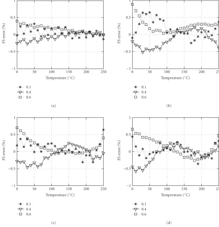
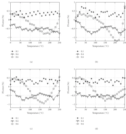
The full-scale (FS) percent error was computed as one hundred times the diﬀerence between the true pressure and the estimated pressure. The FS error at 0◦C, 80◦C, 150◦C, and 250◦C with the applied pressure varying from 0.0 to 0.6 for the four forms of temperature dependencies are plot-ted in Figure 6. Next, in Figure 7, we plotted the FS error for the whole temperature range from 0◦C to 250◦C, at spe-cific values of applied pressure (i.e.,PN =0.1, 0.4, and 0.6),

for NL0 and NL1–NL3. The maximum FS error for the lin-ear form NL0 remains within±0.75%, whereas, in the case of the three nonlinear forms, the maximum FS error remains within±1.0%.

5.2. Estimation of temperature

Plots of true temperature and the estimated temperature as a function ofVN0for the linear (NL0) and the three

(8)

0 80

150 250

0 0.2 0.4 0.6

Normalized pressure −1

−0.5 0 0.5 1

FS

er

ro

r

(%)

(a)

0 80

150 250

0 0.2 0.4 0.6

−0.5 0 0.5 1

FS

er

ro

r

(%)

(b)

0 80

150 250

0 0.2 0.4 0.6

−0.5 0 0.5 1

FS

er

ro

r

(%)

(c)

0 80

150 250

0 0.2 0.4 0.6

−0.5 0 0.5 1

FS

er

ro

r

(%)

(d)

Figure6: Full-scale percent error between the true and the estimated pressures at specific temperatures (0, 80, 150, and 250◦C) with linear and three forms of nonlinear dependencies. (a) NL0. (b) NL1. (c) NL2. (d) NL3.

The FS percent error in estimation of the temperature for the four cases are plotted in Figure 9. For the whole range of temperature variation from 0◦C to 250◦C, the maximum FS error remains within±1% for NL0, NL2, and NL3, and within±2% for NL1. From these observations, eﬀective per-formance of the T-NN is evident. Even though CN0 varies

nonlinearly with temperature in diﬀerent forms of nonlin-ear dependencies, the T-NN is able to estimate the ambient temperature accurately.

From the above findings, it may be concluded that the performance of the MLP model for the estimation of the ap-plied pressure is excellent for the linear form of influence, and satisfactory for the three forms of nonlinear influences of temperature. In a similar application reported by Arpaia et al. [18], an MLP with 43 hidden layer nodes was used and a

maximum error of±2.4% was obtained. In the present study, we have achieved a maximum error of only±1.0% with a small-sized MLP of{2−4−1}architecture (with only 17 weights). This is possible due to careful training of the MLP with the following strategies: (i) proper selection of initial learning rate and the momentum factor, (ii) use of a variable learning parameter (11), and (iii) application of randomly selected patterns from the training set.

(9)

0.1 0.4 0.6

0 50 100 150 200 250

Temperature (◦C) −1

−0.5 0 0.5 1

FS

er

ro

r

(%)

(a)

0.1 0.4 0.6

0 50 100 150 200 250

−0.5 0 0.5 1

FS

er

ro

r

(%)

(b)

0.1 0.4 0.6

0 50 100 150 200 250

−0.5 0 0.5 1

FS

er

ro

r

(%)

(c)

0.1 0.4 0.6

0 50 100 150 200 250

−0.5 0 0.5 1

FS

er

ro

r

(%)

(d)

Figure7: Full-scale percent error between the true and estimated pressures at specific normalized pressures (PN =0.1, 0.4, and 0.6) for the

full range of variation of the ambient temperature. (a) NL0. (b) NL1. (c) NL2. (d) NL3.

6. AN INTERPOLATION SCHEME

Pereira et al. [11] have made extensive study on the rel-ative performance of diﬀerent methods in fitting a curve to sensor’s dataset. Their dataset is one dimensional, that is, the sensor output (pressure readout) is a function of the SCI output. Using diﬀerent interpolation methods, for example, Newton’s, splines, polynomial, and NNs, they showed that the NN-based interpolation scheme outper-forms other methods. When the data set is highly non-linear, the NN-based scheme usually performs much bet-ter than the other methods. The main advantage of the NN-based curve fitting is its excellent extrapolation

capa-bility due to nonlinear processing of multivariate data. Af-ter successful training of the NN, it provides lower er-rors outside the calibration range of the sensor than the polynomial extrapolation. Relative performance of diﬀ er-ent methods of curve-fitting techniques are provided in Table 4 (taken from [11]). Here, the “Poly. Degree” values for the NN row correspond to the number of hidden layer nodes.

We present a polynomial-based interpolation scheme of data fitting of 2D sensor data, and compare its performance with the NN-based model. Here, the sensor data has two in-dependent variables: ambient temperature (x1) and

(10)

True Estimated

0.35 0.4 0.45 0.5 0.55 Normalized SCI output at zero pressure 0 Normalized SCI output at zero pressure 0 Normalized SCI output at zero pressure 0 Normalized SCI output at zero pressure 0

Figure8: The true temperature and the estimated temperature by the T-NN model with linear and three forms of nonlinear dependencies. (a) NL0. (b) NL1. (c) NL2. (d) NL3.

pressure (y). Let the polynomial model of the sensor be given by the coeﬃcients of the model to be determined. The dataset consists of 13 ×5 measurement points corresponding to 13 measurements for each of the five temperature values of 0, 60, 120, 180, and 240◦C. Using Gauss-Newton method, the training data was fitted with the polynomial model. The coeﬃcients of the model are estimated by least squares method.

The average mean square error (MES) between the true and estimated pressures is defined as

MSEavg=

perature values,Ndatpts=13 for the thirteen measurements,

Ptruis the true pressure, andPestis the estimated pressure by

the model. The MSEavgin dB for diﬀerent degrees of

(11)

NL0 NL1

0 50 100 150 200 250

Temperature (◦C) −2.5

−2 −1.5 −1 −0.5 0 0.5 1 1.5

FS

er

ro

r

(%)

(a)

NL2 NL3

0 50 100 150 200 250

Temperature (◦C) −2.5

−2 −1.5 −1 −0.5 0 0.5 1 1.5

FS

er

ro

r

(%)

(b)

Figure9: Full-scale percent error in estimation of temperature by the T-NN model with linear and three forms of nonlinear dependencies. (a) NL0 and NL1. (b) NL2 and NL3.

Table4: Relative performances of diﬀerent methods in fitting a curve to a dataset. The “Poly. deg.” values for the NN row correspond to the number of hidden layer nodes (taken from [11]).

Methods No. of points Max. rel. error(%) Poly. deg. σ×10−2

Newton’s 10 11.5 9 1.7

15 31.2 14 5.6

Splines 10 14.2 3 2.3

15 11.6 3 1.7

Polynomial 10 11.5 9 1.8

15 9.6 9 1.3

NN 10 4.8 6 0.96

15 4.5 5 1.0

Table5: The MSEavgfor diﬀerent degrees of the polynomial model

and the NN model withNtrgset=5. The last-row values indicate the

number of coeﬃcients/weights in the model.

NL form J=3 J=4 J=5 NN model NL0 −43.40 −45.35 −46.99 −51.83 NL1 −41.92 −44.75 −46.77 −49.67 NL2 −46.87 −46.72 −46.51 −50.42 NL3 −45.17 −46.07 −46.55 −49.73

10 15 21 17

degree of the polynomial model is increased. However, for J > 5, there is no substantial improvement in the MSEavg

of the polynomial model. The MSEavg for the P-NN model

is found to be less than that of the polynomial model for the linear (NL0) and the three nonlinear temperature dependen-cies (NL1–NL3).

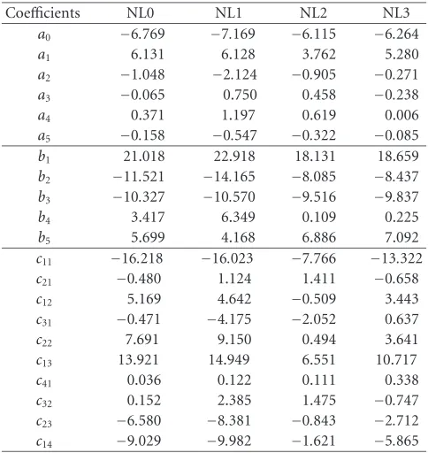
The estimated coeﬃcients for the linear (NL0) and the three nonlinear temperature dependencies (NL1–NL3) for the polynomial model of degree of five (J=5 with 21 coeﬃ -cients) are provided inTable 6. All subsequent comparisons are made based on this polynomial model.

The FS percent error for the polynomial model (J=5) at specific normalized pressure values covering the entire tem-perature range are plotted inFigure 10. Similar plots for the P-NN model are shown in Figure 7. Comparing these two figures, one can see that the FS percent error for the P-NN model is less than that of the polynomial model for the linear (NL0) and the three nonlinear dependencies (NL1–NL3).

(12)

Table 6: The estimated coeﬃcients of the polynomial model

(Ntrgset=5 andJ=5) for linear (NL0) and three nonlinear

temper-ature dependencies (NL1–NL3).

Coeﬃcients NL0 NL1 NL2 NL3

a0 −6.769 −7.169 −6.115 −6.264

a1 6.131 6.128 3.762 5.280

a2 −1.048 −2.124 −0.905 −0.271

a3 −0.065 0.750 0.458 −0.238

a4 0.371 1.197 0.619 0.006

a5 −0.158 −0.547 −0.322 −0.085

b1 21.018 22.918 18.131 18.659

b2 −11.521 −14.165 −8.085 −8.437

b3 −10.327 −10.570 −9.516 −9.837

b4 3.417 6.349 0.109 0.225

b5 5.699 4.168 6.886 7.092

c11 −16.218 −16.023 −7.766 −13.322

c21 −0.480 1.124 1.411 −0.658

c12 5.169 4.642 −0.509 3.443

c31 −0.471 −4.175 −2.052 0.637

c22 7.691 9.150 0.494 3.641

c13 13.921 14.949 6.551 10.717

c41 0.036 0.122 0.111 0.338

c32 0.152 2.385 1.475 −0.747

c23 −6.580 −8.381 −0.843 −2.712

c14 −9.029 −9.982 −1.621 −5.865

(NL1–NL3) temperature dependencies. From the original training dataset, the 13 data points corresponding to 240◦C were removed. Thus, the training data consists of 13×4 data points corresponding to 13 data points from each of 0, 60, 120, and 180◦C (Ntrgset=4).

The NN model, P-NN, was trained with these datasets and a set of weights were obtained for each of the linear (NL0) and nonlinear dependencies (NL1–NL3). Similarly, with a polynomial degree of 5 (J = 5), a set of coeﬃcients of the polynomial model were estimated by using Gauss-Newton method with least squares (for NL0–NL3). The ap-plied pressure was estimated by the P-NN model and the polynomial model using P-NN weights and polynomial co-eﬃcients, respectively. The FS error between the true and the estimated pressures at specific temperature values of 210, 220, 230, and 240◦C for the linear (NL0) and non-linear temperature dependencies (NL1–NL3) are plotted in Figure 11. In this figure, the top row corresponds to the NN model and the bottom row corresponds to the polynomial model.

It may be noted that both the P-NN model and the poly-nomial model have seen data covering only temperatures from 0◦C to 180◦C. FromFigure 11, superior performance of the P-NN model over the polynomial model for temper-ature range of 210◦C–240◦C is evident. In particular, for the linear dependency (NL0), the FS error of the P-NN model remains within±1% (similar to that of the previous case). However, for nonlinear dependencies (NL1–NL3), the maxi-mum FS error remains between +5% and−2%. On the other hand, in the case of the polynomial model, as the

tempera-ture increases from 210◦C to 240◦C, the FS error increases from−3% to−10% for the linear dependency (NL0). The performance for NL1 is the worst for the polynomial model. As the temperature increases from 210◦C to 230◦C, the FS er-ror increases from−5% to−12%, and it becomes more than −15% at 240◦C. For NL2 and NL3, the maximum FS error remains within−13% and−8%, respectively.

Performance comparison between the P-NN model and the polynomial model for the entire range of tempera-ture at specific values of normalized pressure are plotted in Figure 12. In this figure, the top row corresponds to the P-NN model while the bottom row corresponds to the polynomial model. Superior extrapolation capability of the P-NN model is evident in this figure. For the entire range of temperature (0◦C−250◦C), the FS error for linear dependency (NL0) re-mains within±1% for the P-NN model. For the temperature range from 0◦C to 200◦C, the FS error is larger in the poly-nomial model compared to that in the P-NN model. Beyond 200◦C, the performance of the polynomial model is much worse than the P-NN model for the linear and nonlinear de-pendencies (NL0–NL3).

The average MSE, MSEavg, in dB was computed for the

P-NN model and the polynomial interpolation model (Ntrgset=

4 andJ=5) and are provided inTable 7. For the temperature range from 0◦C−250◦C, in comparison toTable 5(Ntrgset=5

andJ =5), a substantial degradation of MSEavgcan be seen

for the polynomial model. On the other hand, although there is a degradation for the NN model, it is not severe. In partic-ular, in the case of the P-NN model there is not much change in the MSEavg for the linear dependency (NL0) compared

with the previous case (Table 5).

For the temperature range from 0◦C−200◦C, the MSEavg

is comparable to that ofTable 5for both the P-NN and poly-nomial models. This fact indicates that the performance of the polynomial model is satisfactory for interpolation, but its performance severely deteriorates in the case of extrapo-lation, whereas the performance of the NN model is found to be superior than the polynomial model for both interpo-lation and extrapointerpo-lation of the sensor data.

7. AN IMPLEMENTATION SCHEME

Due to the rapid decrease in unit cost and fast increase in on-chip capabilities, MCUs have been used in various intelligent embedded systems. An implementation scheme of the MLP-based CPS model using an MCU is depicted in Figure 13. The SCI converts the change in capacitance of the CPS due to the applied pressure into an equivalent voltage level. This analog SCI output voltage is passed through an analog-to-digital converter (ADC). The analog-to-digital temperature informa-tion is similarly obtained from the knowledge of VN0 (i.e.,

(13)

0.1 0.4 0.6

0 50 100 150 200 250

−0.5 0 0.5 1

FS

er

ro

r

(%)

(a)

0.1 0.4 0.6

0 50 100 150 200 250

−0.5 0 0.5 1

FS

er

ro

r

(%)

(b)

0.1 0.4 0.6

0 50 100 150 200 250

−0.5 0 0.5 1

FS

er

ro

r

(%)

(c)

0.1 0.4 0.6

0 50 100 150 200 250

−0.5 0 0.5 1

FS

er

ro

r

(%)

(d)

Figure10: Full-scale percent error between the true and estimated pressures for the polynomial model (J = 5) at specific normalized pressures (PN =0.1, 0.4, and 0.6) with full range of variation of the ambient temperature. (a) NL0. (b) NL1. (c) NL2. (d) NL3.

MLP are stored in the EEPROM of the MCU. With the avail-able hardware, such as adders and multipliers of the MCU, the MLP-based model can be implemented and the digital readout of the applied pressure can be displayed through the bus interface circuit.

To estimate the ambient temperature from the sensor characteristics itself, we propose the following scheme. In practical use of a CPS, there is only one output signal (the SCI output VN) corresponding to the measurand (applied pressure). Therefore, appropriate provisions are to be made to obtain the signals separately for estimation of the temper-ature and the pressure. The online estimation of pressure us-ing the NN-based scheme can be carried out in a

measure-ment phase which consists of one t est and one p est cy-cle. In thet est cycle, the ambient temperature is estimated, whereas in thep est cycle the applied pressure is estimated.

Duringt est cycle, provision is made to separate the CPS from the applied pressure, and the SCI output VN0

corre-sponding to the zero pressure is then recorded. From the knowledge ofVN0, the ambient temperature can be estimated

using the T-NN. Next, during the p est cycle, the pressure is applied to the CPS, and the SCI outputVN is recorded. Now, using the recorded values ofVN0andVN, the applied

(14)

210

Figure 11: Full-scale percent error between the true and estimated pressures at specific temperatures (210, 220, 230, and 240◦C) with diﬀerent forms of nonlinear dependencies. (a) and (e) NL0; (b) and (f) NL1; (c) and (g) NL2; and (d) and (h) NL3. The top row corresponds to the NN model and the bottom row corresponds to the polynomial model (J=5). Both models were trained withNtrgset=4.

However, if the environmental temperature variation is not frequent, then thet est cycle need not be carried out in each measurement phase, but only at regular intervals. The esti-mated temperature of the precedingt est cycle (saved in the RAM of the MCU) can be used to estimate the applied pres-sure in the current meapres-surement phase.

8. CONCLUSIONS

Smart sensors operating in harsh environments should be capable of providing accurate readout and autocompensa-tion of the nonlinear influence of the environmental pa-rameters on its response characteristics. For this purpose, we have proposed a novel NN-based technique for

(15)

0.1 0.4 0.6

0 100 200

Temperature (◦C) −15

Figure12: Full-scale percent error between the true and the estimated pressures at specific normalized pressures (PN=0.1, 0.4, and 0.6) for

the full range of variation of the ambient temperature. (a) and (e) NL0; (b) and (f) NL1; (c) and (g) NL2; and (d) and (h) NL3. The top row corresponds to the NN model and the bottom row corresponds to the polynomial model (J=5). Both models were trained withNtrgset=4.

Table7: The MSEavgfor the polynomial model (Ntrgset = 4 andJ = 5) and the NN model with linear (NL0) and the three nonlinear

temperature dependencies (NL1–NL3).

NL form Temperature 0–250

◦_C _{Temperature 0–200}◦_C

Poly. model NN model Poly. model NN model

NL0 −30.01 −50.17 −45.33 −51.48

NL1 −25.02 −42.66 −42.97 −49.67

NL2 −28.11 −38.07 −44.87 −50.93

NL3 −34.70 −46.12 −46.19 −50.45

The performance of the NN model was compared with that of a polynomial interpolation scheme with a

(16)

CPS SCI

Figure13: A scheme of a MCU-based implementation of the pres-sure sensor NN model.

especially for extrapolation of data. A scheme for an MCU-based implementation of the proposed NN-MCU-based models is also provided. Such NN-based models may be applied to other types of sensors to incorporate intelligence in terms of mitigating the nonlinear dependency of their response char-acteristics on the environmental parameters.

ACKNOWLEDGMENT

The authors would like to express their sincere thanks to the anonymous reviewers whose positive and constructive com-ments helped to enhance the quality and presentation of this paper.

REFERENCES

[1] P. T. Kolen, “Self-calibration/compensation technique for microcontroller-based sensor arrays,” IEEE Trans. Instrum.

Meas., vol. 43, no. 4, pp. 620–623, 1994.

[2] P. Hille, R. Hohler, and H. Strack, “A linearisation and com-pensation method for integrated sensors,”Sensors and

Actua-tors B, vol. 44, no. 2, pp. 95–102, 1994.

[3] M. Yamada and K. Watanabe, “A capacitive pressure sensor interface using oversampling∆−Σdemodulation techniques,”

IEEE Trans. Instrum. Meas., vol. 46, no. 1, pp. 3–7, 1997.

[4] K. F. Lyahou, G. van der Horn, and J. H. Huijsing, “A non-iterative polynomial 2-D calibration method implemented in a microcontroller,”IEEE Trans. Instrum. Meas., vol. 46, no. 4, pp. 752–757, 1997.

[5] X. Li, G. C. M. Meijer, and G. W. de Jong, “A microcon-troller-based self-calibration technique for a smart capacitive angular-position sensor,”IEEE Trans. Instrum. Meas., vol. 46, no. 4, pp. 888–892, 1997.

[6] G. Bucci, M. Faccio, and C. Landi, “New ADC with piecewise linear characteristic: case study-implementation of a smart humidity sensor,” IEEE Trans. Instrum. Meas., vol. 49, no. 6, pp. 1154–1166, 2000.

[7] W. J. Kulesza, A. Hultgren, J. McGhee, M. Lennels, T. Bergan-der, and J. Wirandi, “An in-situ real-time impulse response auto test of resistance temperature sensors,” IEEE Trans.

In-strum. Meas., vol. 50, no. 6, pp. 1625–1629, 2001.

[8] S. Haykin, Neural Networks, Maxwell Macmillan, Ontario, Canada, 1994.

[9] L. F. Pau and F. S. Johansen, “Neural network signal under-standing for instrumentation,” IEEE Trans. Instrum. Meas., vol. 39, no. 4, pp. 558–564, 1990.

[10] P. Daponte and D. Grimaldi, “Artificial neural networks in measurements,” Measurement, vol. 23, no. 2, pp. 93–115, 1998.

[11] J. M. Dias Pereira, P. M. B. Silva Girao, and O. Postolache, “Fitting transducer characteristics to measured data,” IEEE

Instrum. Meas. Mag., vol. 4, no. 4, pp. 26–39, 2001.

[12] J. C. Patra, G. Panda, and R. Baliarsingh, “Artificial neural network-based nonlinearity estimation of pressure sensors,”

[13] J. C. Patra, A. C. Kot, and G. Panda, “An intelligent pressure sensor using neural networks,” IEEE Trans. Instrum. Meas., vol. 49, no. 4, pp. 829–834, 2000.

[14] J. C. Patra, A. van den Bos, and A. C. Kot, “An ANN-based smart capacitive pressure sensor in dynamic environment,”

Sensors and Actuators A, vol. 86, no. 1-2, pp. 26–38, 2000.

[15] J. M. Dias Pereira, O. Postolache, and P. M. B. Silva Girao, “A temperature-compensated system for magnetic field mea-surements based on artificial neural networks,” IEEE Trans.

Instrum. Meas., vol. 47, no. 2, pp. 494–498, 1998.

[16] A. Carullo, F. Ferraris, S. Graziani, U. Grimaldi, and M. Parvis, “Ultrasonic distance sensor improvement using a two-level neural-network,” IEEE Trans. Instrum. Meas., vol. 45, no. 2, pp. 677–682, 1996.

[17] G. Y. Tian, “Design and implementation of distributed mea-surement systems using fieldbus-based intelligent sensors,”

IEEE Trans. Instrum. Meas., vol. 50, no. 5, pp. 1197–1202,

2001.

[18] P. Arpaia, P. Daponte, D. Grimaldi, and L. Michaeli, “ANN-based error reduction for experimentally modeled sensors,”

Jagdish C. Patra was born in Nabarang-pur, Orissa, India, in 1957. He obtained his B.S. (with honours) and M.S. degrees, both in electronics and telecommunication engi-neering, from Sambalpur University, India, in 1978 and 1989, respectively. He received his Ph.D. degree in electronics and commu-nication engineering from the Indian In-stitute of Technology, Kharagpur, in 1996. After the completion of his B.S. degree, he

worked in various R&D, teaching, and government organizations for about 8 years. In 1987, he joined the Regional Engineering Col-lege, Rourkela, Orissa, as a Lecturer, where he was promoted to an Assistant Professor in 1990. In April 1999, he went to the Tech-nical University, Delft, the Netherlands, as a Guest Teacher (Gast-docent) for six months. Subsequently, in October 1999, he joined the School of Electrical and Electronic Engineering (EEE), Nanyang Technological University (NTU), Singapore, as a Research Fellow. Currently, he is serving as an Assistant Professor in the School of Computer Engineering, NTU, Singapore. His research interests in-clude intelligent signal processing using neural networks, fuzzy sets, and genetic algorithms in the area of data security, sensor networks, image processing, and bioinformatics. He is a Member of IEEE, USA, and Institution of Engineers, India.

(17)

Narendra S. Chaudharireceived his B.Tech. (with distinction), M.Tech., and Ph.D. de-grees from the Indian Institute of Tech-nology, Mumbai, India, in 1981, 1983, and 1988, respectively. After completing his B.Tech. degree in electrical engineering, he worked on the design of microprocessor-based electronic controllers in the Elec-tronic Controls Division of Larsen and Toubro Ltd, Mumbai, in 1981. After

receiv-ing his Ph.D. degree in computer engineerreceiv-ing, he was involved in graduate-level training for the defense scientists (Ministry of De-fense, Government of India) till 1998. He was a Visiting Professor in Southern Cross University, NSW, Australia, and Freie Universi-tat, Berlin. Currently, he is with School of Computer Engineering, Nanyang Technological University, Singapore, as an Associate Pro-fessor since 2001. His research interests are in the areas of neural networks, computational learning, and optimization algorithms. He has more than 100 research publications to his credit. He is a Fellow of Institution of Electronics and Telecommunication Engi-neers, India, Chartered Engineer of Institution of EngiEngi-neers, In-dia, Senior Member of Computer Society of InIn-dia, and member of many professional societies, including Singapore Computer Soci-ety, and Pattern Recognition and Machine Intelligence Association, Singapore.

Amitabha Dasobtained his B.Tech. degree with honours in electronics and electrical communication engineering from the In-dian Institute of Technology, Kharagpur, and his Ph.D. degree in computer engi-neering from the University of California, Santa Barbara. He has been with the School of Computer Engineering, Nanyang Tech-nological University, Singapore, since 1992, where he is currently an Associate Professor.