Volume Rendering Transfer Function Design Based on eXtreme Gradient Boosting for Fast Visualization

2019 International Conference on Computational Modeling, Simulation and Optimization (CMSO 2019) ISBN: 978-1-60595-659-6

Volume Rendering Transfer Function Design Based on eXtreme Gradient

Boosting for Fast Visualization

Qing-mei WANG, Tong ZOU, Han CUI and Peng SHI

National Center for Materials Service Safety, University of Science and Technology Beijing, Beijing 100083, China

*Corresponding author

Keywords: Volume rendering, Transfer function, XGBoost, Fast visualization.

Abstract. Volume visualization has been widely used to simulate and observe complex data in the fields of science, engineering, biomedicine, etc. One central topic of volume visualization is the transfer function (TF) of volume rendering. By setting TF, users design the mapping of voxels to optical properties of 3D datasets. However, the design of TF is usually a blind process. How to classify all volume data accurately and design a suitable TF fleetly is the key to improve the efficiency of volume rendering. In this paper, we propose a new TF design approach based on extreme gradient boosting (XGBoost) algorithm for fast visualization. First, the features are extracted from 3D volume data. Then we use the XGBoost model to classify the volume data and design TF. Finally, we assign the optical properties to the voxels to express and reveal the relevant features of dataset. This approach can help users to render the volume data efficiently. It has been tested and achieved satisfactory result.

Introduction

Volume rendering is an important algorithm to express the volume data. It directly projects a 3D data field into a translucent 2D image. The algorithm is widely used in the visualization of scientific computing, engineering computing, medical scanning and other fields. In the volume rendering algorithm, transfer function (TF) is an extremely important component, which is responsible for converting the values of volume data into optical features, such as opacity, color, etc. Opacity determines whether voxels of volume data are visible in the rendered image. Voxels of interest are usually assigned a higher opacity than other voxels. The color of voxels in the rendering result can also be determined by TF. By assigning different colors to different categories of voxels, the internal structure of the volume data can be observed more clearly. In summary, TF determines the quality of the rendering result.

network, which improves the efficiency of human-computer interaction and the automation of designing TF [5]. Zhang et al. proposed to use general regression neural network (GRNN) to design TF [6]. GRNN combines the characteristics of the RBF neural network and the probability network. In their study, the amplitude of the curvature and the eigenvalue of the second-order directional derivative matrix are used as the input of the neural network. The visualization parameters are adjusted by evaluating the results of the output rendering. Although the neural network is continuously improved during the training process and the classification results become better and better, it is difficult to obtain the best classification result. Local optimization may occur during the update process. In addition to the neural network, support vector machine (SVM) is also used to classify the volume data [7]. SVM trains the entire training data set. When the training is completed, the optimal classification result can be obtained and the classification error is guaranteed to be global minimum. Compared to neural networks, SVM requires fewer samples and shorter time of training process. However, SVM is more sensitive to missing values which increases the cost of data preprocessing.

In general, the main problem with TF is the lack of guidance during the design process. More importantly, the classification of dataset is not accurate and efficient enough. These problems reduce the efficiency of volume rendering. In order to get the objects of interest in the data field, users often need a lot of attempts to adjust the visualization parameters to get a reasonable TF.

In this paper, we propose a method of volume rendering transfer function design based on extreme gradient boosting (XGBoost) algorithm. XGBoost is a new machine learning classification algorithm that has been successfully used in text classification, item classification, behavior prediction, risk assessment and other fields. In the algorithm, the appropriate regularization is included in the objective function to control the complexity of the model. Besides, the algorithm sets the default direction for missing values to handle sparse data. Therefore, we apply XGBoost to classify volume data and design transfer function.

Methods

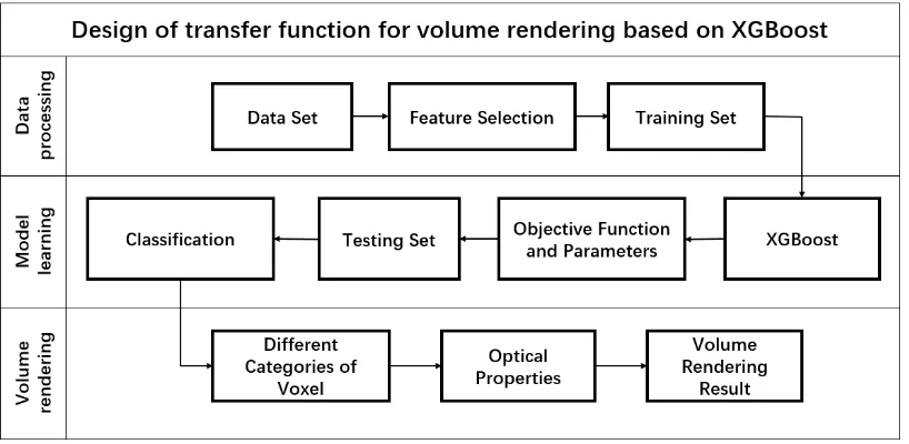
Figure 1 shows the general diagram of the transfer function design method based on XGBoost. It is divided into three parts: data processing, model learning and volume rendering.

Figure 1. Design of transfer function for volume rendering based on XGBoost.

Data Processing

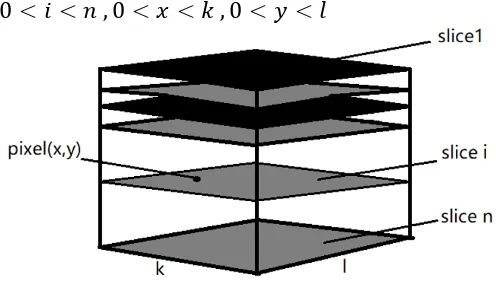
v(x, y, i) = 𝑝𝑖(𝑥, 𝑦) 0 < 𝑖 < 𝑛 , 0 < 𝑥 < 𝑘 , 0 < 𝑦 < 𝑙 (1)

Figure 2. Structure of Volume Data.

The most intuitive features of voxel only include its position and gray value. However, in machine learning, the higher the dimension of features, the stronger the ability to scatter data. It is possible to make data separable by mapping from low to high dimensions. In order to improve the ability of volume data classification, we extract some representative features according to the position and gray value of the dataset.

Gradient Magnitude. For 3D volume data, we usually assume that the same substance has similar scalar values while different substances have different values. Therefore, the scalar values of voxels at the boundary will vary greatly, which will cause the change of gradient magnitude. In 3D space, the formula (2) for calculating the gradient amplitude is as follows.

∥ ∇𝑣(𝑥, 𝑦, 𝑧) ∥= 1₃√(𝐹𝑥)2+ (𝐹𝑦)2+ (𝐹𝑧)2 (2) For the discrete 3D data field, the gradient can be calculated by the central difference method.

{

𝐹𝑥 =1₂[𝑣(𝑥 + 1, 𝑦, 𝑧) − 𝑣(𝑥 − 1, 𝑦, 𝑧)]

𝐹𝑦 = 1₂[𝑣(𝑥, 𝑦 + 1, 𝑧) − 𝑣(𝑥, 𝑦 − 1, 𝑧)]

𝐹𝑧 =1₂[𝑣(𝑥, 𝑦, 𝑧 + 1) − 𝑣(𝑥, 𝑦, 𝑧 − 1)]

(3)

Second Derivative. Using higher derivative as the design basis of transfer function can extract the characteristics of data field more accurately. When the gradient of boundary surface reaches its maximum, the second derivative of the gradient direction becomes 0. So we can use the minimum of second derivative to distinguish the boundary of substance in volume data. The formula (4) for calculating the second derivative is as follows.

𝐷_∇𝑣2 _{𝑣 =} ∇𝑣

∥∇𝑣∥∇(∥ ∇𝑣 ∥) (4)

Smoothness. Smoothness is a feature that reflects the continuity of surface shape of substance. It can be calculated by standard deviation, as shown in formula (5).

𝑠_{𝑣(𝑟,𝑠,𝑡)} = 1 −_1+𝜎1

𝑣2 , 𝜎𝑣 = √

∑ ∑ ∑𝑧+1 [𝑣(𝑟,𝑠,𝑡)−𝑣̅]2

𝑡=𝑧−1 𝑦+1

𝑠=𝑦−1 𝑥+1

𝑟=𝑥−1

27 (5)

Curvature. Curvature is an important feature of surface. To a certain extent it determines the shape of substance. Analyzing the curvature of data can enhance the classification effect of the model. K₁

and K2 represent the maximum and minimum bends [8]. The calculation method of curvature is shown in formula (6).

𝐾₁ = 𝑇−√2𝐹₂2−𝑇2 , 𝐾₂ = 𝑇+√2𝐹₂2−𝑇2 (6) where T is the trace of matrix G and F is the corresponding Frobenius norm. To obtain the matrix

𝐺 = ∇𝑛𝑇_{𝑃 (7)} where n = −g/|g|, P = I − nnT and g = [𝜕𝑣_𝜕𝑥𝜕𝑣_𝜕𝑦𝜕𝑣_𝜕𝑧]T.

Local Histogram. Local histogram reflects the relationship between voxels and other voxels around it. The information obtained from the local histogram can effectively help the model to classify the data. We calculated the entropy H and moments m_n of the local histogram. The formulas (8-10) are as follows.

ℎ(𝑖) =∑ ∑ ∑𝑧+1𝑡=𝑧−1𝑔(𝑖)

𝑦+1 𝑠=𝑦−1 𝑥+1

𝑟=𝑥−1

27 , 𝑔(𝑖) = {1 𝑣(𝑟, 𝑠, 𝑡) = 𝑖, 𝑖 ∈ [0,255]_{0 𝑜𝑡ℎ𝑒𝑟𝑤𝑖𝑠𝑒} (8)

H = − ∑𝑖=𝑣𝑚𝑎𝑥ℎ(𝑖)𝑙𝑛ℎ(𝑖)

𝑖=𝑣𝑚𝑖𝑛 (9)

𝑚𝑛 = ∑𝑖=𝑣𝑖=𝑣𝑚𝑎𝑥_𝑚𝑖𝑛 𝑖𝑛ℎ(𝑖) (10)

max

v and v_max represent the maximum and minimum gray values of local histograms in voxel domain, respectively.

Model Learning

After obtaining the voxel features of the samples, we use the data as training set to train the XGBoost model. XGBoost is an improvement of GBDT algorithm. GBDT only uses first derivative when optimizing, while XGBoost uses both first derivative and second derivative. At the same time, the algorithm takes the complexity of decision tree as a regular term in the objective function, which effectively avoids over-fitting. Assuming that the data to be classified is composed of K classes, these data were randomly segmented according to the ratio of 9:1 of training set and test set. Then we trained the model by 10-folds cross-validation to get K classification results. Finally, the prediction model is obtained.

Volume Rendering

The XGBoost model classifies each voxel and generates a matrixA x y z( , , ). The numerical range of the matrix is between [1,K] and K is the number of classifications specified by users. We generated

K transfer functions F(1), (2),..., ( )F F k and mapped the classification results {1, 2,..., }k to the corresponding transfer functions. We use F m v_c( , ) to represent the color transfer function and

( , ) a

F m v to represent the opacity transfer function, where m represents the result of classification and v represents the scalar value of voxels. The voxel synthesis formula (11) is as follows [9].

{𝐶𝑐𝑢𝑟 = 𝐶𝑠ℎ𝑒𝑙𝑡𝑒𝑟+ (1 − 𝛼𝑠ℎ𝑒𝑙𝑡𝑒𝑟)𝐹𝑐(𝑚, 𝑣)

𝛼𝑐𝑢𝑟 = 𝛼𝑠ℎ𝑒𝑙𝑡𝑒𝑟+ (1 − 𝛼𝑠ℎ𝑒𝑙𝑡𝑒𝑟)𝐹𝛼(𝑚, 𝑣) (11)

Case Study

We have validated our schemes with medical CT and MRI volume datasets. All tests are conducted on a system equipped with a 2.8GHz Intel Core i7 CPU, 16G of main memory and Intel Iris Plus Graphics 655 with 1.5G of video memory. In the following subsections, we will provide some rendering results.

(a) (b)

Figure 3. Visualization of CT-foot (256x256x256) dataset with two different visual angle.

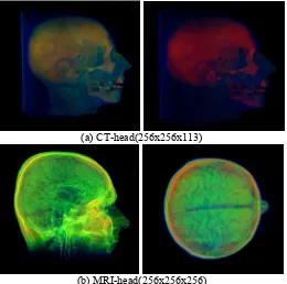
Figure 4 (a) and (b) show the rendering results of a head CT dataset (256x256x113) and a head MRI dataset (256x256x256). By observing the rendering results, we can see that both skull and soft tissues parts are distinguished. The fold structures of soft tissues can also be displayed.

(a) CT-head(256x256x113)

(b) MRI-head(256x256x256)

Figure 4. Rendering results: (a) is a visualization of CT-head which displays the skull; (b) is a visualization of MRI-head which displays the soft tissues.

Figure 5 is a tooth CT dataset (256x256x161). Considering that the difference between the gray values of this dataset is smaller than other datasets, we use a larger max_depth for model training. Finally, the different structures such as enamel, dentin, pulp are displayed.

(a) (b)

Conclusion

In this paper, we proposed a new transfer function design approach for volume rendering based on XGBoost. Firstly, we extract the features of volume data, such as gradient magnitude, second derivative, smoothness and so on. After obtaining the voxel features, we use the data as training set to train the XGBoost model by 10-folds cross-validation. The XGBoost model classifies each voxel and generates its classification. Finally, we assign the optical properties to the voxels to obtain the corresponding results. Experiments show that the proposed framework can render volume data with high quality. In addition, XGBoost algorithm is used to avoid over-fitting and reduce the calculation time in the classification process.

In the future research, it is aimed to develop a transfer function design method with more automation and higher quality, which can be used for medical visualization to render volume data more efficiently.

Acknowledgement

This paper is financially supported by National Key R&D Program of China (No. 2017YFB0203703).

References

[1] Ji-Wei Chen, Yin F, Jun-Li X, et al. Transfer Function Design Based on K-means Clustering[J]. Computer and Modernization, 2014.

[2] Atwan A. 3-D ISODATA and Region Growing technique for segmentation a true color Visible Human dataset[C]//International Conference on Informatics & Systems. 2012.

[3] Cen Zi-yuan, Li Bin, Tian Lian-fang. High dimensional transfer function design based on K-means ++ for volume visualization [J]. Journal of Computer Applications, 2012, 32(12): 3404-3407.

[4] Tzeng F Y, Lum E B, Ma K L. A novel interface for higher-dimensional classification of volume data[C]// Visualization, 2003. VIS 2003. IEEE. IEEE, 2003.

[5] Zhou Hui, Zhang You-sai, Li Yuan-jiang. Design of multi-dimensional transfer function for volume rendering based on RBF neural network[J]. Computer Engineering and Applications, 2016, 52(22):180-184.

[6] Zhang J W, Sun J Z. Adaptive transfer function design for volume rendering by using a general regression neural network [rendering read rendering][C]//International Conference on Machine Learning & Cybernetics. 2003.

[7] Li Jin, Zhou Lu-lu, Yu Hong, et al. Classification of Volume Data Based on Support Vector Machine[J]. Journal of System Simulation, 2009, 21(2):452-456.

[8] Kindlmann G, Whitaker R, Tasdizen T, et al. Curvature-Based Transfer Functions for Direct Volume Rendering: Methods and Applications[C]//Visualization, 2003. VIS 2003. IEEE. IEEE, 2003.