Modeling, Simulation and Control Solutions For Mechatronics Design of Solar Light Tower

(1)

ISSN 2348 – 7968

Modeling, Simulation and Control Solutions For Mechatronics

Design of Solar Light Tower

Mohammed M. K.1,2 ,Farhan A. Salem 1,3

1_{Dept. of Mechanical Engineering, College of Engineering, Taif University, 888, Taif, Saudi Arabia.}

2_{El-Minia University, Faculty of Engineering, Production Eng. & Design Dept.,}

3_{Alpha center for Engineering Studies and Technology Researches, Amman, Jordan.}

Abstract

As an option to conventional light tower (LT) that uses

ICE as electricity generator source, an integration of LT design and PhotoVoltaic (PV) panels resulting in Solar

light tower (SLT),this paper proposes a new generalized

and refined model for Mechatronics design of pure standalone SLT and some considerations regarding design,

modeling and control solutions. The selection, design and

integration of main subsystems including mechanical structure, electric DC machines and controls are proposed. The SLT system is designed to operate in two modes manual and automatic. The proposed SLT system model consists of seven main subsystems, each subsystem, is mathematically described and corresponding Simulink sub-model is developed, then an integrated generalized model of all subsystems is developed, and is developed to allow designer to have the maximum output data (numerical and graphical) to select, test and evaluation the overall SLT system and each subsystem outputs characteristics and performance, for desired overall and/or either subsystem's specific outputs, under various PV subsystem input operating conditions, to meet particular SLT system requirements and performance. The obtained results show the simplicity, accuracy and applicability of the presented designs and models to help in Mechatronics design of SLT systems .

Keywords: Mechatronics, Photovoltaic (PV) system, Solar Light Tower (SLT), Modeling, simulation.

1. Introduction

In last years an increasing attention and more importance are dedicated to researches in the fields of alternative machines using internal combustion engines as electricity generator source, and corresponding fuel consumption economy and reduction of related emissions. As an option to conventional light tower (LT) using ICE as electricity generator source, an integration of LT design and PhotoVoltaic (PV) panels resulting in Solar light tower

(SLT). it uses the PV panel as electricity generator to

convert the irradiance from sunlight into electricity, to generate its own power for lightening and for storing in batteries, all the power needs are supplied 100% by the PV

panel subsystem, it generates electricity and provides light

without noise, any fuel consumption and any related emissions, the SLT system is designed to replace used

diesel powered light tower, and can be applied at locations where fuel availability and mains powered electricity is not available or is too expensive to implement

Considering that theessential characteristicandthe keyto

success in Mechatronics system design is a balance

between two sets of skills modeling/analysis and

experimentation/hardware implementation skills, where Modeling, simulation, analysis and evaluation processes in Mechatronics design consists of two levels, sub-systems models and whole system model with various sub-system models interacting similar to real situation[1], this paper proposes a new generalized and refined model for Mechatronics design of pure Standalone SLT and some considerations regarding design, modeling and control

solutions, that can be applied to help in facing the two top

challenges in developing Mechatronics Standalone SLT systems; early identifying system level problems and ensuring that all design requirements are met.

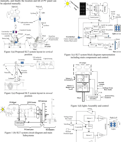
The proposed whole SLT system model consists of seven main subsystems, each subsystem, is to be mathematically described and corresponding Simulink sub-model is developed, then an integrated generalized model of all subsystems is developed, finally the subsystems models and the whole SLT system model, are to be tested and analyzed for desired system requirements and performance, under various PV subsystem input operating conditions. The proposed SLT system and each subsystem design and integration, layout, circuit and block diagram representations are shown in Figure 1.

Features and specifications of proposed SLT design:The proposed design is to result in the following: Better light distribution and area coverage. Towed-portable on it own two wheels SLT. Mast is easily cranks up, stowed and extends, using either manual or controlled winch. The lamps may be adjusted in the desired direction up, down, left or right; manually and automatically, less weight, cost

efficient, aerodynamically efficient design.Set-up; simple,

easy and fast: easy set-up by one person in less minimum

time counted in minutes; tow the SLT unit to the desired site location, park the unit, deploy the jack stands, adjust solar panel to face sun, aim the lights at the desired target for illumination, deploy the lighting mast, and turn the

lighting system on. Operating Modes; the proposed design

can operate with two modes; automatically On/Off using a programmable lighting system that uses photocell and

Manual operating mode for light when it is required.Zero

(2)

ISSN 2348 – 7968

For achieving these features, the below specifications are selected; Maximum height of SLT tower 8 m, Maximum height SLT unit with mast stowed 2 m, Overall length with mast stowed 6 m, Overall trailer frame width with fenders 3 m, 4 X 1000w Metal Halide Floodlight, mounted on light cross member in cuboid housing.

2. Selection, design and integration of each subsystem and whole SLT system

The proposed SLT system and corresponding model consists of seven main subsystems, in particular; PV panel, DC/DC converter, battery bank, three separate DC actuating machine, control units and mechanical structure with its dynamics sub-model, each subsystem,

2.1 Subsystems selection, design and integration.

Light subsystem; For better light distribution and area

coverage, a (4 X 1000 Watt) Metal halide floodlight lamps are selected, it produce an intense white light, has high luminous efficacy of around 75 - 100 lumens per watt, with 6000 to 15000 working hours. [1-2] these to be supported with quick disconnect fixtures and plug in ballasts. For a 4x1000w tower light, can illuminate areas greater than 4500m² at an average 20 lux [3]. As shown in Figure 1(d), each lamp is proposed to be located in gasket with high reflectivity surface with polishing and oxidation treatment. a pair of lamps are mounted on light cross member from both sides (see Figure 1) and fixed using handle bolts, and both pairs of lamps to be located in a cuboid housing, that in turn mounted on motor shaft with gears, finally, all this assembly are mounted on other, second, motor shaft with gears, the first motor allows light subsystem to rotate vertically up and dawn with limits from zero to 45 deg ,whereas the second motor allows the whole first assembly ( with first motor) to rotate horizontally right and left with limits from zero to 90 deg in either direction. The whole lights sub-system assembly to be adjusted to rotate up, down, left or right, both manually and automatically: manually, where each of the four lights can be adjusted manually to desired direction, by loosening the handle bolts on the lamp fixtures and aiming them in the desired direction, and automatically through user interface,(Joystick or Keypad) applying simple PI-controller with corresponding control components, as shown in Figure 1(d)

Actuator subsystem; 24 V DC machines as prime

movers are a suitable, available, and simple to interface choice.

Sensors subsystem; for position control, limit switches

and/or potentiometers are suitable, available, and simple to interface choice.

PV subsystem; consists of PV panel, DC/DC

Converter/charge controller, with MPPT algorithm, to

charge the 24Volt battery bank, for 12-hour nightly run time, the PV subsystem layout, circuit and diagram representation are shown in Figure 1(b) Figure 1(c). The PV panel is to be designed to provide the required power, with manually adjustable-tilt and location around the mast base, to face the sun rise and sunset, the assembly is mounted on a round base with slots for adjusting PV panel location. To reduce the effects of wind speed and corresponding aerodynamic and lift forces, an 3D octagon (see Figure 1(a)) with base greater than upper surface with slope of 45 degrees, can be used as base (chassis) to support the PV panel and move it to any of it's eight surfaces, facing the sun also as shown in Figure 1, the 3D octagon, can be used as housing cover for the SLT base with battery bank, DC/DC converter charge controller, control and circuitry.

Trailer subsystem; the Mast with lamps (tower) are

mounted on trailer, that includes axle springs for smooth towing on highways and jobsites, a standard steel fenders are to be used. To provide support for wind speed (wind stability), the design include a four telescopic outriggers and jack, these are shown in Figure 1(b).

Mast subsystem; is designed to easily raised up and

extends to the vertical position to 8 m in height, by dual easily hand-operated or controlled electric winch, with

corresponding, cables and pulleys.Safety considerations;

To ensure the safety, the mast is to be supported with-locking pin at the base of the pivot post that lock automatically and user will hear it “snap” into place[5].Also a sensing device (limit switch or potentiometer) for ensuring maximum motions limits of 90 degrees and height to be used.

Control unit subsystem; Microcontroller type (PIC

18FXX) , with corresponding drive and voltage regulator is a suitable, available, inexpensive, easy to program choice, suitable for controlling the motions of motors, the control system layout is shown in Figure 1(c)

User interface subsystem; can be located above the top

surface of the octagon; it can be selected to be a joystick, keypad, pushbutton or display for data inputting and displaying.

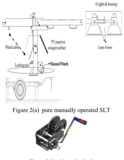
2.2 Pure manual SLT system design

The proposed design of SLT can further be simplified and reduced in cost, to have the construction shown in Figure 2(a), by removing control systems and corresponding components, resulting in pure manually operated SLT. In this design, the mast is rise manually, by hand-operated winch shown in Figure 2, also, each of the 4 lights can be adjusted manually to desired direction, by loosening the handle bolts on the lamp fixtures and aiming

them in the desired direction, also the assembly with 4

(3)

ISSN 2348 – 7968

manually, and finally the location and tilt of PV panel can be adjusted manually.

Up-Dawn Up-Dawn

Right-Left

Round base with slots to adjust PV panel location Octagon

User interface

Right-Left

Battery bank

Lights position control & 2 motors

Controls & Circuitry

Converter & charge

controller PV panel Winch

Figure 1(a) Proposed SLT system layout in vertical

position 2 DC machines for

lights positioning 4 Lights & housing

Winch Locking pin Winch cable

User interface

PV panel on octagon surface

Figure 1(a) Proposed SLT system layout in stowed

position

Control systems

Bat.

IB

VB

+-Vref or VV

D I,V

PV Cell/panel DC/DC Converter

PV Control system

SLT Control system

SLT subsystem

VV Positions

Figure 1 (b) SLT system circuit diagram and main Subsystems

IPV

VPV

Control system1

I

B

a

tt

ery

V

Iload

Drive 1

Control 2 Motor1

Volt.Reg. _Sensors

Load & hor. position

(User interface)

Control ; Desired Lamps Position, Winch control

Load & Vert. position Motor2

Lightsand dynamics On/Off

Switch

Drive 2 Winch Gears

Pulley

Mastand dynamics

Up

-Da

w

n

Sensor

D

LDR Sensor

From controller

Figure 1(c) SLT system block diagram representation including main components and control.

4 Lamps

Control and circuitry Motor 1

UP-DAWN

Motor 2 Right-Left

desired Pos. control On/Off

switch

Voltage from Bat. bank V.R.

Mast

Figure 1(d) lights Assembly and control

Drive

Motor 1 Gears

Controller

sensor

Motor 2 Gears

sensor

Lights Desired

Position input Voltage from Bat. bank

Volt.Reg.

Right-Left

Up

-D

awn

(4)

ISSN 2348 – 7968

Figure 1 (a)(b)(c)(d) Proposed SLT system design, layout, circuit and block diagram representations of main overall

system and subsystems, including; PV panel, DC/DC converter, battery bank, DC actuators and controls.

4 Lights & housing

Manual Winch Locking pin

Winch cable octagon surfacePV panel on Lamps fixtures

Figure 2(a) pure manually operated SLT

Figure 2(b) Manual winch

3. Modeling of SLT system

The proposed SLT system and corresponding model consists of seven main subsystems, each subsystem, is to be mathematically described and corresponding Simulink sub-model is to be developed, then an integrated generalized model of all subsystems is to be developed.

3.1 Mathematical bases of lamps

Lumens are converted to watts, as described next; The

power P in watts is given by Eq.(1) and the luminance Ev

in lux (lx) is given by Eq.(2)

/ V

P  



(1)





)

2

( 10.76391 /

v lx V

E   A

(2)

Where: ΦV the luminous flux in lumens, (lm) and η :the

luminous efficacy in (lm/W), A: the surface area A in

square m, for Metal halide lamp η= 75-100 lm/W and ΦV

=75*103_-105_lm.

For a spherical light source, the area A is given by Eq.(3)

_A__{4· ·}__r2₍₃₎

The energy consumption (kWh) = System Input Wattage (kW) x Hours of Operation/Year

Hours of Operation/Year = Operating Hours/Day x Operating Days/Week x Operating Weeks/Year

3.2 Modeling and simulation of the PV cell, module, panel and array

PV system is a whole assembly of solar cells, connections, protective parts, supports etc. The basic

device of a PV system is the single PV cell. Cells are

hermetically sealed under toughened, high transmission glass to produce highly reliable, weather resistant modules that may be warranted for up to 25 years. PV system naturally exhibits a nonlinear I-V and P-V characteristics

which vary with the radiant intensity β and cell

temperature T.In the dark, the I-V output characteristic of

a solar cell has an exponential characteristic similar to that of a diode [6-7], therefore, the simplest equivalent circuit of a PV solar cell consists of a diode, a photo-current, a parallel resistor expressing a leakage current, and a series resistor describing an internal resistance to the current flow, this all is shown in Figure 1(b) and Figure 4(a), this

equivalent circuit is called a single diode model, a more

accurate model is called double diode model and shown in

Figure 4(b) . The diode determines the I-V characteristics of the cell (Figure 4(e,f)) [11]. A general mathematical description of I-V output characteristics for a PV cell has been studied for over the pass four decades and can be found in different resources including [7-28].

The output net current of PV cell I, and the V-I

characteristic equation of a PV cell, is found by applying

the Kirchoff’s current law (KCL) on the equivalent

simplified single diode circuit shown in Figure 4(d). The net output current is the difference of two currents; the

light-generated photocurrent Iph and diode current Id

[7-28]., and is given by Eq.(4)

ph d

II I (4) The light-generated photocurrent Iph is generated by the

incident light and directly proportional to the sun

irradiation β and operating temperature, Iph isgiven by

Eq.(5).









₁₀₀₀

ph sc i ref

I  I K T T  (5) The cell’s short-circuit current ISC,is the current through

the solar cell when the voltage across the solar cell is zero

(see figure 3(e)(f)), ISC is calculated when the voltage

equals to zero I (at V=0) = Isc, at T= 25°C and the solar

insolation β=1kW/m2_{, given in datasheet specifications of}

PV panel.

The diode current Id is given by Eq.(6).

( )

I I 1

S q V IR

NKT d s e



 

   

 

(5)

ISSN 2348 – 7968

Based on this, the basic equation for output net current of

PV cellI, of the PV cell represented as single diode with series resistance RS and without shunt resistance RSH,

shown in Figure 3(c), is obtained by substituting Eqs.(5) and Eq. (6) in Eq.(4) , this gives Eq.(7):

( )

I I I S 1

q V IR NKT ph s e



 

  _  _

  (7) The basic equation given by Eq. (7) does not represent the

actual I-V characteristics of practical and real operation of PV cell, because in the real operation of the solar cell some losses exist, to get a more real behavior and to pick

up these losses in real PV cell, a third current based on Rs

and Rsh, called shunt current IRsh and given by Eq.(8), is

added, with these additions the corresponding equivalent circuit diagram is as shown in Figure 3(a) [25], and the net current of the cell will be given by Eq.(7), this equation shows that the output current generated depends on the PV

cell voltage V, solar irradiance β on PV cell, and ambient

temperature T. Eq.(9) describes the single-diode model

presented in Figure 4(e), this model offers a good compromise between simplicity and accuracy and for simplicity is used and modeled in this paper. Characteristic I-V curve of a practical photovoltaic device and the three remarkable points, is shown in Figure 4(e).

S RSH sh

V

R

I

R





(8)









( )

I

I I I 1

I I 1

1000

S

d RSH q V IR

S NKT

ph s

sh q V IR ph

S NKT

sc i ref s

sh

I

V R I

e

R

V R I

I I

I K T T e

R                        _  _   (9)

The diode reverse saturation current IS, is constant under

the constant temperature T, and found by setting the

open-circuit condition, using Eq. (7), let I = 0 (no output

current) and solve for IS, gives Eq.(10). The diode reverse

saturation current Is, varies as a function of the

temperature T, as given by Eq.(11).

mod

1 SOC ₁

Sc sc

s

qV qV

NKT N KAT

S I I le I u I

e _e 

               _ _ (10) 3 1

3 1 1

( ) ( ) g ref g ref qE T T NKT S S ref qE T T NKT

S S

ref

T

I T I e

T

I T I e

T  _                         _ _      _ _   (11)

The power produced by a single PV cell is not enough for general use, where, each solar cell generates around 0.5V, therefore the PV cells are connected in series-parallel configuration on modules, where series connections for high voltage requirement and in parallel connections , or PV panels consisting of one or more PV modules, to produce desired power output. Panels can be grouped to

form large photovoltaic arrays. The term array is usually

employed to describe a complete power-generating unit,

consisting of any number of PV modules and panels. PV

module mathematical model ; The current output of given PV module, considering the number of parallel and series

connections of cells NP , NS, is given by Eq.(12).

( )

I I I 1

S S P IR V _P q S N N S NKT

P ph P s

sh

N V _{R I}

N

N N e

R         _  _     (12) The maximum PV voltage; Since the PV cell efficiency is

insensitive to variation in shunt resistance RSH , the effect

of parallel resistance RSH can be neglected (Figure 4(c) in

Eq. (9), the maximum PV voltage can be represented by

Eq. (13).

ln ph s

s s

I I I

NKT V IR q I      _ _   (13) Open circuit voltage Vo; Corresponds to the voltage drop

across the diode (p-n junction), when it is traversed by the

photocurrent Iph when the generator current is I = 0. It

reflects the voltage of the cell in the night, and given by

Eq. (14):

ln ph 0

o

s

I NKT

V for I

q I    _ _    (14) The power delivered by a PV system of one or more

photovoltaic cells is dependent on the irradiance, temperature, and the current drawn from the cells. The power output of a PV system is given by Eq.(16):

*

P V I



(16) Maximum Power Point, MPP, is the operating point at which the power is maximum across the load and given by Eq.(17):

max max* max

P V I (17) Efficiency (Maximum) of solar cell is the ratio between

the maximum power Pmax and the incident light power, and

given by Eq.(18), where Pinis taken as the product of the

solar irradiation of the incident light (G=β/1000),

measured in W/m2_{, with the surface area (}_A_{) of the solar}

(6)

ISSN 2348 – 7968 max

out in in

P P

  (18)

* 1000 in

A

P   (19) Fill factor (FF) :The departure of the I-V characteristic of

a real cell from that of a perfect cell is measured by the fill

factor (FF) of the cell, it is a measure of quality of the solar cell, It is calculated by Eq.(20),by comparing the

maximum power (Pmax) to the theoretical power (Pth) that

would be output at both the open circuit voltage and short circuit current together[ 18]

max max

*

th sc o

P P

FF

P I V

  (20)

3.2.1. Maximum Power Point and MPP tracking

The power delivered by a PV system of one or more photovoltaic cells is dependent on the irradiance,

temperature, and the current drawn from the cells. The power output of a PV system is given by:

*

P V I



With incremental change in current ΔI ,and voltage ΔV,

the modified power is given by Eq.(30), by solving and then ignoring small terms, Eq.( 30) simplifies to Eq.(31),

since no changes power at peak point, that is ΔP=0,by

manipulating and in the limits , will result in Eq.(32)



P P

 

V  V

 

* I I



(30)

* *

P V V I I

     ( 31)

V dV V

I dI I

 _ _{ }



(32) Maximum Power Point, MPP, is the operating point at which the power is maximum across the load and given by:

max max

*

max

P



V

I

Figure 4 (a) single diode (exponential) model of the PV

model Figure 4 (b) Double diode (exponential) model of PV Cell

Figure 4 (c) single diode (Appropriate,) model of PV Cell Figure 4 (d) simplified Ideal single diode model of

(7)

ISSN 2348 – 7968

Figure 4(e) Characteristic I-V curve of a practical

photovoltaic device and the three remarkable points: short

circuit (0, Isc), maximum power point (Vmp, Imp) and

open-circuit(Vo, 0)[17]

Figure 4(f) Typical characteristic I-V and P-V curve of a practical photovoltaic device and the

three remarkable points [18]

3.3 Modeling and simulation of PV cell ; module, panel and array

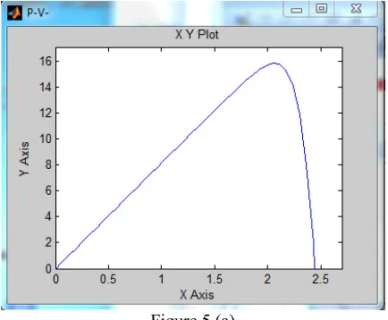
Based on Eq.(12), PV cell Simulink model Simulink model is shown as sub-model of the generalized SLT system model and shown in Figure 7(b) the mask model is shown in Figure 7(c)

For PV subsystem sub-model model shown in Figure 7(b), by defining parameters including number of series and

parallel PV cells (NS,NP,), the corresponding PV module

can be tested and evaluated, this model can be used to develop required PV module, panel or array. Running this

model for defined parameters listed in Table-2 at standard

operating conditions; will result in P-V and I-V

characteristics shown in Figure 5, these curves show, this

is 3.926 Watt PV cell, ISC = 8.13 A , Vo= 0.6120V , Imax

=7.852 A , Vmax =0.5 V, (MPP = Imax * Vmax =7.852

*0.5=3.926).

Figure 5 (a)

Figure 5 (b)

Figure 5(a)(b) P-V and I-V characteristics of PV module consisting of four series PV cells

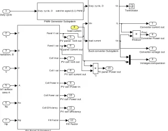
3.4 Modeling and simulation of the buck converter

In this paper, Buck converter is a suitable DC/DC

converter to be used with PV system and tested to result in

constant desired output voltage of 24 V to be fed to DC

actuators. Buck converter is used for voltage step-down; it

is power converter which DC input voltage is greater than DC output voltage. A simplified buck converter circuit diagram is shown in Figure 1(b) as subsystem of whole SLT circuit diagram . The exact control of output voltage is accomplished by using a Pulse-Width-Modulation

(PWM) signal to drive the buck converter MOSFET-switch

ON or OFF, by controlling the switch-duty cycle D, based on this, if the principle of conservation of energy is applied then the ratio of output voltage to input voltage is given by Eq.(33):

*

out in on

out in

in out on off

V I T

D V D V D

V  I    T T (33)

Where: Iout and Iin, : the output and input currents. D : the

duty ratio (cycle) and defined as the ratio of the ON time of the switch to the total switching period. The PWM generator is assumed as ideal gain system, In this paper, for transfer function block diagram representation, the duty

cycle of the PWM output will be multiplied with gain Kv=

KD, This equation shows that the output voltage is lower

than the input voltage; hence, the duty cycle is always less than 1. The mathematical model of buck converter in its

two switch positions (ON , OFF), can be derived applying

Kirchoff's voltage and current laws. The simplified

(8)

ISSN 2348 – 7968

differential equations given by Eq.(34), The dynamics when the ideal switch is ON are given by Eq.(35). The buck converter subsystem Simulink model and mask, shown as sub-model of the generalized SLT system model are shown in Figure 7(d), the mask model is shown in Figure 7(c)

1

( R R )

, 0 , :

( R R L )

L

in o on L L L

o L

o on L L L

di

V V i i

dt L _{t dT} _{Q ON}

dV di

v i i

dt dt  _ _{ } _  _{ }   _ _ _ _  (34) 1 ( )

, 0 , :

1 ( ) * L in o o L o di V v

dt L _{t dT} _{Q ON}

dv

i v

dt C R

 _ _  _{ }   _ _  (35)

3.5 Photovoltaic panel-Converter (PVPC) system model

The developed both Simulink models of PV panel and buck converter are integrated to result in single Simulink model and mask shown as sub-model of the generalized SLT system model in Figure 7(e)

3.6 Actuators subsystem modeling

The proposed design of SLT is developed with three actuating systems; two separate DC motors are used to adjust light-assembly direction to rotate up, dawn, right and left to result in better area coverage, also, and a controlled electric winch with corresponding, cables and pulleys is used to raise ( crank up) the mast to vertical location. In both cases a suitable position sensor is to be used to detect and limit actuator's motion.

3.6.1 Modeling the light-assembly DC motors and sensor subsystems

The actuating machines most used in Mechatronics motion control applications are DC machines (motors). PMDC motor a suitable, available and easy to control actuator for light-assembly. In [29-33] introduced tested and verified a detailed derivation of refined mathematical model and corresponding Simulink model of DC machine and sensor, based on these, the open-loop transfer function of the PMDC is given by Eq.(36), In the following

calculation the disturbance torque, T, is all torques

including coulomb friction, and given by

(T=Tload+Tf).Dynamics of potentiometer can be

represented using Eq.(37),

  2   

( ) ( ) ( ) / ( ) ( ) Lights open in t open

a a equiv equiv a a b t

s

G s

V s

K n

G s

s L s R J s b s L s R T K K

             (36)

 

_

_ (Voltage change) (Degree cha gn e) pot out pot

pot out tpot

V t K t

V t K t       (37)

The geometry of the mechanical part determines the moment of inertia, the light-assembly can be considered to be of the cuboid shape with dimensions; width, b= 0.3 m , depth, L= 0.5 m and height h=0.5 m , whereas, the Mast

can be considered to be a rod with length L=6 m and mass

M. For light assembly, the total equivalent inertia, Jequivand

total equivalent damping, bequivat the armature of the motor

with gears attached is calculated as given by Eq.(38).Considering the light-assembly of rectangle m rotating a round a perpendicular axis through it's center ,the inertia is calculated by Eq.( 38). these values are to be

substitute in Eq.(31) to replace motor's J and b, to result in

open loop transfer function of DC motor with light load attached 2 2 2 1 2 2 1 2 , ,

(b h )

12

load

equiv m gear Load

equiv m Load

M J

N

J J J J

N

b b b

N        _ _       _ _   (38)

Each DC machine must generate torque required to overcome all load torques, these load torques are to be mathematically modeled and simulated, then integrated with the DC machine Simulink model. An acceleration is required to move the light-assembly to desired position, this added torque is calculated based on that the sum of torques acting at pivot lifting joint is equal to mast moment

of inertia, Jlight multiplied by the angular acceleration, as

given by Eq.(39),

2 2

* (

*

b h )

12 light J M T T



   (39)

Considering aerodynamic Drag force opposing the motion

of the light-assembly due to air drag, the aerodynamic drag

force is function of light-assembly linear velocity, ν and

given by Eq.(40):

2

aerod d

F  0.5 * * A*C *





vehicl (40)

(9)

ISSN 2348 – 7968 2

aerod d

1

T * * A*C * *

2  vehicle rr

 

 _ _ (41)

Where: Cd : Aerodynamic drag coefficient characterizing

the shape of the mast and can be calculated using the expression given by Eq.(42),where S: frontal area of light-assembly , square shape with length, 0.5 m and width of 0.5 m

aerod 2

F 0.5 D

C

S



 (42)

Considering the aerodynamics lift force, Flift; that iscaused

by pressure difference between the light-assembly front and back side, and is given by Eq.(43), Where: B : SLT

reference area. CL: The coefficient of lift, and can be

calculated using the expression given by Eq.(44):

_{0.5* *} _{* *} 2

lift L

F   C B  (43)

2 0.5 L

L C

A





(44)

Where: L: lift,the air density (kg/m3_{) at STP,}_ρ_{=1.25, A:}

light-assembly frontal area (length* width= 0.25 M). V: light-assembly velocity.

The DC machine subsystem Simulink model with sensors and load dynamics, are shown in Figure 7(f)(g) , also is shown as mask sub-model of the generalized SLT system model in Figure 7(a)

To determine the electric battery capacity, and correspondingly design the of Photovoltaic panel with series and parallel connected cells, it is required to estimated energy required by each DC machine, the required power in kW that each DC machine must develop at stabilized operation can be determined by multiplying the total force with the velocity of the light-assembly, and given by Eq.(45):

(

) *

*

Total Total

P

 

F





F



(45)

Electrical power (in watts) in a DC circuit can be calculated by multiplying current in Amps and V is voltage, and given by Eq.(46):

P= I x V (46)

3.6.2 Winch subsystem modeling

Electrically powered winch is used to raise the mast from stowed position to vertical position, an electric DC motor is selected as actuator to generate desired power, the mathematical and Simulink model of DC motor are given

by Eq.(36). The total equivalent inertia, Jequivand total

equivalent damping, bequivat the armature of the DC motor

with gears attached is calculated as given by Eq.(38). Since, the geometry of the mechanical part determines the moment of inertia, the Mast can be considered to be rod of

length L= 6 and mass m =1500 kg, The moment of inertia

can be found by computing the integral, given by Eq.(47)

2

/2 3 3

/2 2

/2 /2

/ 8 1 2

3 3 12

l

Mast l

l

x m l

J x sdx s s ml

sl

  _





_

   (47)

An acceleration is required to move the mast from a level position, this added torque is calculated based on that the sum of torques acting at pivot lifting joint is equal to mast

moment of inertia, JMast multiplied by the angular

acceleration, as given by Eq.(48),

2

* 1

12 *

Mast

T J

T ml

 



(48)

Also, referring to Figure 6, for winch lifting a mast, the torque required is given byEq.(49). Considering aerodynamic Drag force opposing the motion of the mast due to air drag, given Eq.(40), The aerodynamics torque is

given by Eq.(41), where: Cd : characterizing the shape of

the mast and can be calculated using the expression given by Eq.(42),where S: frontal area of mast , assumed to be

cylindrical , with length, 6 m and width of 0.3 m.

Considering the aerodynamics lift force, Flift; that iscaused

by pressure difference between the mast front and back side, and is given by by Eq.(43), where: B : reference

area. CL: A: frontal area (length* width= 1.8 M). Referring

to figure 7, for the worst case, the torque required at lifting

joint to raise the mast vertically, and to hold Mast at a

given distance from lifting joint can be found by Eq.(50) . Performing, torque balance about lifting joint, given by Eq.(51), Substituting T from Eq.(50) in Eq.(51), gives Eq.(52):

T= r.M.g.cos(θ) (49)

T= F*L= M*g*L (50)

0

T    F L T



(51)

T



M g L

 

(52) The DC machine subsystem Simulink model and mask

with sensor of winch system, are shown as sub-model of the generalized SLT system model in Figure 7(f) the mask model is shown in Figure 7(a)

Mast mass

Gears

Motor

Mast mass

F= M*g F= M*g* cosθ

T

Figure 6 Torque calculations

(10)

ISSN 2348 – 7968

3.7 Control system modeling

Different control algorithms, including PI, PID , can be proposed to control the overall SLT system output performance in terms of output angular position, as well as, controlling output characteristics and performance of PVPC subsystem to meet desired output voltage or current under input working operating conditions.

PI controller: because of its simplicity and ease of

design, PI, PD and PID controllers is widely used in

variable speed applications and current regulation. In this

paper PI controller will be applied for achieving desired outputs characteristics of PVPC subsystem and meeting desired output speed of overall SLT system , where separate PI controllers configurations are to be applied to control the PVPC subsystem and overall SLT system to achieve desired outputs of position, voltage and load currents, it is important to notice that, in the proposed SLT model, PI controller can be replace with any other suitable control algorithm.

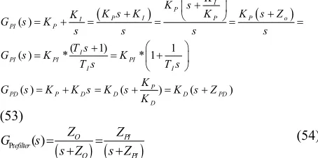
The PI and PD controllers transfer function in different

forms are given by Eq.(53). The controller's pole , zero

will affect the response, mainly the PI zero given by; Zo

=-KI/KP, will inversely affect the response and should be

cancelled by prefilter, while maintaining the proportional

gain (KP), the prefilter transfer function is given by Eq.(54)

, the placement of prefilter is shown on generalized model[34].

   

( )

( 1) 1

( ) * * 1

( ) ( ) ( )

I P

P I P P o

I

PI P

I

PI PI PI

I I

P

PD P D D D PD

D

K

K s

K s K K K s Z

K

G s K

s s s s

T s

G s K K

T s T s

K

G s K K s K s K s Z

K

 _ 

 

 _ _ 

     

 



  _  _

 

     

(53)



 



Prefilter( ) O PI

O PI

Z Z

G s

s Z s Z

 

  (54) The Suggested control system to control the actuators of

SLT system are shown as sub-model in SLT model in Figure 7 (h)

PVPC subsystem controllers :The power delivered by a

PV system is dependent on the irradiance β, temperature T,

and the current drawn from the cells V. To maximize a PV

system's output power, it is necessary continuously tracking the maximum power point (MPP) in the I-V characteristic of the PV system (see Figures 4(e,f)) , a switch-mode power converter, can be used to maintain the PV’s operating point at the Maximum Power Point MPP, The Maximum Power Point tracker MPPT, does this by controlling the PV array’s voltage or current independently of those of the load.

Perturb and observe algorithm; A detailed Simulink

model of perturb and observe algorithm is shown in Figure

7(i).The VPV and IPV are taken as the inputs to MPPT unit,

duty cycle D is obtained as output. In this perturb and observe algorithm a slight perturbation is introduced to the system. Due to this perturbation the power of the module changes. If the power increases due to the perturbation then the perturbation is continued in that direction, after the peak power is reached the power at the next instant decreases and hence after that the perturbation reverses. When the steady state is reached the algorithm oscillates around the peak point [35]

Also, A PI controllers, also can be used to control PV panel characteristics, where two separate PI controllers are used, first PI current controller shown in Figure 7(g), is used to match motor-current with required Load-torque (Variations) current to overcome, where both currents are compared and the difference is fed to PI controller to generate converter's output current in accordance with Duty cycle to match and generate required load current. A second PI voltage controller shown in Figure 7(g), used to control the converter's output voltage to match desired output voltage, by comparing desired converter output voltage (24 V) and actual converter's voltage, the difference is fed to PI controller to control the buck converter MOSFET switch according calculated duty cycle to result in desired voltage[35-36].

4. Smart day night control and simulation

LDR can be used as day-night sensing device, to switch lights of SLT system ON and off, LDR is interfaced to corresponding microcontroller (e.g.PIC 10FXXX) input pin, that will control the drive circuit, that in turn switch lights ON and OFF, algorithm flow chart is shown Figure 7(a), circuit simulation in Proteus is shown in Figure 7(b)(c) .

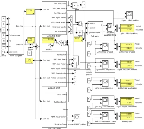
5. Proposed generalized whole SLT system Simulink model

The proposed generalized SLT system model is developed by integrating all subsystems sub-models, is shown in Figure 8(a)

6. Testing, analysis and evaluation

(11)

ISSN 2348 – 7968

acceleration all versus time, and in Figure 9(b) are shown response curves of consumed current, load current , motor generated torque and load torque all versus time. Correspondingly response curves of actuator responsible for Horizontal right-left motions are shown in Figure 9(c)(d) and for actuator responsible for mast motions, are shown in Figure 9(e)(f).

In Figure 9 is shown the plots relating the vertical and horizontal motions, in particular, positions, speeds, and accelerations of SLT mast and of lambs assembly versus , where in Figure 10(a) is shown the relation between angular positions of both vertical and horizontal motions,

in Figure 10(b) is shown the relation between linear positions of both vertical and horizontal motions, in Figure 10(c) is shown the relation between linear speeds of both vertical and horizontal motions, , in Figure 10(d) is

shown the plot between angular accelerations of both

vertical and horizontal motions, in Figure 10(e) is shown

the plot of linear acceleration positions of both vertical

and horizontal motions, in Figure 10(f) is shown mast angular position versus time, finally in Figure 10(g) is shown lights assembly center point motion versus time. The simulation output numerical values, of each subsystem and whole SLT system are listed in Table1

Vetical

Horizental

Vetical

Horizental

Currents

HORIZ. angular position

Vetical

Horizental

Vetical

Horizental

Vetical

Horizental

Vetical

Horizental Top Center

point POSITION V_position

H- position

Lights linear speed X1

Y1

Sub system u

Sqrt T

B.

V

Cell surf ace area

Ns

Np

Motor current Conv . I out

Conv Vout

PVPC Subsystem

0.2835

-9.277

Motors powers Mast ANGULAR position

Conv Vout

Conv Iout

VERT. Speed

Mast Motor Current

Time

VERT. Angular position

Masr Motor Power

MAST: UP-DAWN

0.01876

-0.1146

Lights: linear SPEEDS

Conv Vout

Conv Iout1

Motor Current

VERT. linear Speed

VERT. linear Position

VERT. angular Position

VERT. Angular Acceler

Vertical Linear acceler

Vert. Motor Power

Lights: UP-DAWN Conv Iout

Conv Vout

Horiz. linear Speed

Horiz. linear Position

Hor. Motor current

Horiz. angular Position

Horiz. Angular Acceler.

Horiz. Linear acceler

Hor. Motor Power

Lights: RIGHT-LEFT

35.01

100.6

Lights: ANGULAR positions Lights ANGULAR positions

-T-

-K-1

0.1161

-T-,1

-T-,

Lights: linear acceleration Lights: linear SPEEDS

Lights: Angular acceleration

Horiz. VS Vert motors powers

-0.3851

0.234

Lights: Angular acceleration Lights: LINEAR positions

15.09

5.252

Lights: LINEAR positions

-0.05777

0.0351

Lights: linear acceleration -0.2492

72 77.79

24 Nm

Ns A V B

72 T

(12)

ISSN 2348 – 7968

Illumination reading (LDR1 and LDR2) Light sensor

Converting LDR readings Comparator or

PIC corresponing pins

Set RB? to 1

end LDR >= 47

Yes No

Set RB? to 0

Figure 7(a) Flowchart of microcontroller programming (algorithm)

Figure 7(b)(c) day-night sensor circuit simulation in Proteus[38]

cell current P

I V

V

P V

I

Ish

Id Iph Is

8 Fill Factor

7 Cell Efficiency

6 Cell Power out

5 Cell Power in

4 Cell I out 3

Cell Vout

2 Panel I out 1

Panel V out

V1

I12.mat

To File2 P.mat

To File1 V.mat

To File

75

PV module output voltage

0.5

PV cell voltage Module V

[P] Goto [P]

From

Cell P-V

Cell I-V B

B0

1000

1

100 .9

.8

.7

.6 .5

.4 .3

.2

.11 .10

.1

K

.'

PV.mat

.

,.

eu

,

eu

,

''4

''3

''2 ''1

'' N

'

205.7

1 Vo

.

Rs

Ki

Rsh

Tref

1

Isc

q

2.938 6 Np 5

Ns

4 A 3 V

2 B 1

T

(13)

ISSN 2348 – 7968

Figure 8(b) PV cell/panel Simulink model shown as sub-model of the generalized SLT system model

Pout

13 PV panel Power out

12 Fill Factor

11 PV cell efficiency

10

PV cell Power out 9 PV cell Power in

8 PV cell current out

7 PV cell Volt out

6 PV panel current out

5 PV panel Volt out

4 Converter Power out

3 Volatges comparision

2 Converter voltage out

1 Converter current out Terminator

Product

Duty cy cle, D switchin signal (0,1) PWM

PWM Generator Subsystem

T

B

V

A

Ns

Np

Panel V out

Panel I out

Cell Vout

Cell I out

Cell Power in

Cell Power out

Cell Ef f iciency

Fill Factor

PV Panel Subsystem1

Duty cy cle, D

Vin

load current

Vc

IL

Vo

Buck converter Subsystem

''1 8

load current

7 Np

6 Ns 5 Cell surface

area A 4 V 3 Irradiation, B

2 T 1 Duty cycle

Figure 8(c) The PV-Converter subsystem, including three mask models of three subsystems: PV subsystem, converter subsystem and PWM generator

3 Vo 2 IL

1 Vc Product

Duty cy cle, D switchin signal (0,1) PWM

PWM Generator Subsystem

R/(L*(R+Rc)) 1/(C*(R+Rc)) 1/L

12.02

R/(R+Rc)

1

s

((RL+Ron)+((R*Rc)/(R+Rc)))/L

(R*Rc)/(R+Rc)

R/(C*(R+Rc))

1 s 2

Vin 1 Duty cycle, D

(14)

ISSN 2348 – 7968

Currents

T

B.

V

Cell surf ace area

Ns

Np

Motor current Conv . I out

Conv Vout

PVPC Subsystem T

-72 77.79

24 Nm

Ns A V B

72 T

Figure 8(e) PV Panel-Buck converter mask subsystem of three subsystems PV, Converter and PWM.

Current Torque

EMF constant Kb

angular speed Current

Voltage desired from Voltage controller

Kt

torque constant

-K-rad2mps V=W*r

linear speed 1/n

gear ratio 1

La.s+Ra

Transfer function 1/(Ls+R)

1

Jequiv.s+bequiv

Transfer function 1/(Js+b)

DC_Machinet.mat

Kb

-K-Load Dyn. & Kf

1 s Input V

Anular angle

-K-position sensor

-K-Current sensor

-K-Current required

(15)

ISSN 2348 – 7968

Angle angul ar

speed aerodynamics l ift torque

r*m/2 r*m/2 Coloum Fri cti on aerodaynami c torque,

Load torque

PI Control ler

10 Horiz. Li near acceleration

9 Out1 8 Out2 7 Load orque 6 Motor orque 5 DC machine Current, I

4 Angular HORIZONTAL Posi tion 3

Angul ar HORIZONTAL accel eration

2 Linear HORIZONTAL Position 1

Linear HORIZONTAL speed. 1 -K-rads2mps= R_wheel*(2*pi)/(2*pi). -K-rad2degree n gears -K-angle feedback Kpot

-K-1 La.s+Ra Transfer 1/(Ls+R)3 1 den(s) Transfer 1/(Js + b)3 Saturati on1

rou Rou: The invi ronment ( air) densi ty (kg/m3) 1

-T-Mass_l ights

Manual Switch

-C-M : The mass light-assembly

-K-Kt 1 s 1 s Integrator. -C-H_inertia1=(b^2+h^2) [motor_current] -T-[r1] -T-Kb EMF constant Divi de7 Di vide6 Divi de18 Divide17 Divi de16 Di vide15 Divide14 Divi de,1 du/dt du/dt Deri vati ve 12

Constant

Cd1 Cd : Aerodynamic

drag coeffici ent

CL1 CL: The coeffici ent of l ift

-C-B : underside area

Angular acceleration

Angle- theta

Angl e- degrees

-T-Ang. accel

Add3

A1 A:Cross-secti onal area , where it i s the wi dest, (m2)2

2 1 1. 1 -K-. s+Zo s ,1 r1 Lights radi us

bm 1 Kp 3 Prefilter 2 Controll er 1 Input Vol t,(0 :12)

Figure 8(g) Simulink model of the PMDC machine subsystem used in SLT ( Vertical horizontal and mast actuating DC machines) with load dynamics .

PI Control l er

(Joysti ck )

0:180

6 Hori z. Li near accel er 5

Hori z. Angul ar Accel er.

4 Hori z. angul ar Posi ti on

3 M otor current

2 Hori z. l i near Posi ti on

1 Hori z. l i near Speed

l oad torque Vi n (0:24)

Vert. l i n posi ti on

Vert. Angl . posi ti on VERT . Accel

T orque

SLT _UP7.m at

SLT _UP6.m at SLT _UP4.m at

Zo s+Zo Prefi l ter.

1 1 Prefi l ter PID(s)

PID Control l er1

PI(s) PI Control l er

PD(s) PD Control l er1

Motor current M otor current

Input Volt,(0 :12)

Controller

Pref ilter

Linear HORIZONTAL speed.

Linear HORIZONTAL Position

Angular HORIZONTAL acceleration

Angular HORIZONTAL Position

DC machine Current, I

Motor orque

Load orque

Out2

Out1

Horiz. Linear acceleration

Li ghts sybsystem : RIGHT -LEFT s+Zo s ,1 -K-Kp 1 Conv Vout

(16)

ISSN 2348 – 7968

Figure 8(i)Perturb and Observe Algorithm simulation [35]

PV panel V out PV panel I out

Converter V out Converter I out

2 Conv Vout

1 Conv. I ou

[Conv_current]

Duty cy cle

T

Irradiation, B

V

Cell surf ace area A

Ns

Np

Load current

PV panel current out

PV panel Volt out

Conv erter I out

Conv erter V out

PVPC Subsystem

PI(s)

PI Controller

[panel_Iout]

[Conv_Vout] [panel_Vout]

[Conv_current]

PV_con13.mat [D]

[control]

75 2.161e+004

72 77.79

54.18 7

Motor current 6

Np 5 Ns 4 Cell surface area

3 V 2 B. 1 T

Figure 8(g) Twp separate PI controllers (right and below)for controlling PV output characteristics

0 2 4 6 8

-2 0 2 4

Me

te

r

Vert. LINEAR Speed 

0 2 4 6 8

Me

te

r

Vert. LINEAR Position

0 2 4 6 8

-20 0 20 40

Time(s)



Vert. ANGULAR Acceler. 

0 2 4 6 8

0 20 40 60

Time(s)



Vert. ANGULAR Position

Figure 9(a) vertical up-dawn motion response curves; linear position, angular position, linear speed and angular acceleration all versus time

[Conv_Vout]

[panel_Vout]

V_out_desired

Vout desired

PI(s)

PI Controller1

1.001

0.96

D desired 0.96

D calculated

PV_con11.mat

4 [D]

(17)

ISSN 2348 – 7968

0 2 4 6 8

-10 0 10 20 30

Am

p

e

re

Vert. MOTOR current

0 2 4 6 8

-100 0 100 200 300

Am

p

e

re

Vert. LOAD Current

0 2 4 6 8

-10 0 10 20 30

Time(s)

N/

m

2

Vert. MOTOR Torque

0 2 4 6 8

-5 0 5 10 15

Time(s)

N/

m

2

Horiz. LOAD Torque

Figure 9(b) vertical up-dawn response curves of consumed current, load current , motor generated torque and load torque all versus time

0 2 4 6 8

0 5 10 15

Me

te

r

Horiz. LINEAR Speed _

0 2 4 6 8

0 5 10 15

Me

te

r

Horiz. LINEAR Position

0 2 4 6 8

-100 0 100 200

Time(s)



Horiz. ANGULAR Acceler. _

0 2 4 6 8

0 50 100

Time(s)



Horiz. ANGULAR Position

(18)

ISSN 2348 – 7968

0 2 4 6 8

0 50 100

A

m

p

er

e

Horiz. MOTOR current

0 2 4 6 8

0 50 100

Am

p

e

re

Horiz. LOAD Current

0 2 4 6 8

0 50 100

Time(s)

N/

m

2

Horiz. MOTOR Torque

0 2 4 6 8

-50 0 50

Time(s)

N/

m

2

Horiz. LOAD Torque

Figure 9(d) Horizontal right-left motion response curves of consumed current, load current , motor generated torque and load torque all versus time

0 2 4 6 8

-100 0 100 200 300

M

e

ter

Mast LINEAR Speed 

0 2 4 6 8

0 200 400 600

cm

Mast LINEAR Position

0 2 4 6 8

-50 0 50 100

Time(s)



Mast ANGULAR Acceler. 

0 2 4 6 8

0 20 40 60 80 100

Time(s)



Mast ANGULAR Position

(19)

ISSN 2348 – 7968

0 2 4 6 8

-20 0 20 40 60

A

m

pere

Mast MOTOR current

0 2 4 6 8

-100 0 100 200 300

A

m

pere

Mast LOAD Current

0 2 4 6 8

-50 0 50 100

Time(s)

N/

m

2

Mast MOTOR Torque

0 2 4 6 8

-1 0 1

2x 10

7

Time(s)

N/

m

2

Mast LOAD Torque

Figure 9(f) Mast response curves of consumed current, load current, motor generated torque and load torque all versus time

1 1.1 1.2 1.3 1.4 1.5 1.6 1.7 1.8 1.9 2 70

71 72 73 74 75 76 77 78 79 80

Time (secnd)

M

a

gni

tude

PV Panel-converter outputs

Converter I out Converter V out PV panell V out

0 0.01 0.02 0.03 0.04 0.05 0.06 0.0 0

20 40 60 80 100 120 140 160 180 200

Time (secnd)

M

a

gni

tu

de

PV Panel-converter outputs

Converter I out Converter V out PV panell V out

(20)

ISSN 2348 – 7968

0 0.05 0.1 0.15 0.2 0.25 0.3 0.35 0.4

0 0.2 0.4 0.6 0.8 1

Time (secnd)

M

agn

itu

d

e

Time Series Plot:

PI 'Voltage' controller signal

Figure 9(h) PI control signal

Figure 10(a) the plot of relating angular positions of both

vertical and horizontal linear speeds Figure 10(b) the plot of relating vertical and horizontal motions linear positions of both

(21)

ISSN 2348 – 7968

Figure 10(d) the plot of relating angular accelerations of

both vertical and horizontal motions Figure 10(e) the plot of relating positions of both vertical and horizontal motions linear acceleration

Figure 10(f) mast angular position versus time Figure 10(g) lights assembly center point motion versus

time

Table 1(a) Simulation results of each subsystem and whole SEDDMRP system for straight line motion

PVPC system inputs

PV cell outputs PV Panel outputs Converter outputs DC machinee outputs

β 300 Voltage 0.5 V Voltage 75 V Voltage 72 Input voltage 24 V

T 75 Current 1.37 A Current 46.01 Current 77.79 Right-left

output Ang. position.

90

D 0.5 Fill factor 0.1374 P-out 5594.4 Up-dawn

output Ang. position

45

A 0.0025 Power out 0.6835 Mast Ang.

position

90

Ns 150 Power in 0.5

(22)

ISSN 2348 – 7968

Conclusions

A new generalized and refined model for Mechatronics design of pure standalone solar light tower and some considerations regarding design, modeling and control solutions are proposed. The proposed SLT system model consists of eight main subsystems, each subsystem, is mathematically described and corresponding Simulink sub-model is developed, then an generalized whole SLT system model is developed by integrating all sub-models, the generalized model is developed to allow designer to have the maximum output data (numerical and graphical) to select, model, simulate, analyze and evaluation the overall SLT system and each subsystem outputs characteristics and performance, for desired overall and/or either subsystem's specific outputs, under various PV subsystem input operating conditions, to meet particular SLT system requirements and performance. The obtained results show the simplicity, accuracy and applicability of the presented designs and models to help in Mechatronics design of SEV system .

Table 2 Nomenclature and nominal characteristic of SLT subsystems

Lights DC machine parameters

Vin=24 V Input voltage to DC machine

Kt=1.188 Nm/A Motor torque constant

Ra = 0. 1557Ω Motor armature Resistance

La=0.82 MH Motor armature Inductance,

Jm=0.271 kg.m2 Geared-Motor Inertia

bm=0.271 N.m.s Viscous damping

Kb=1.185 rad/s/V Back EMF constant,

n=1 Gear ratio

Jequiv kg.m2 The total equivalent inertia,

bequiv N.m.s The total equivalent damping,

Kpot =0.2667 Tachometer constant, for

right-left motion

Kpot1=0.0.5333 Tachometer constant, for

up-dawn motion

ω=speed/r, rad/s Shaft angular speed rad/sec

Tshaft The torque produced by motor

η The transmission efficiency

Tshaft The torque, produced by the

driving motor

Mast DC machine parameters

M,m, Kg The mass of the mast

Kt=3.1882Nm/A Motor torque constant

Ra = 1 Ω Motor armature Resistance

La=1 MH Motor armature Inductance,

Jm=1 kg.m2 Geared-Motor Inertia

bm=1 N.m.s Viscous damping

Kb=3.1882rad/s/V Back EMF constant,

Cd =0.80 Aerodynamic drag coefficient

CL The coefficient of lift, with

values

Cr=0.5 The rolling resistance

coefficient

ρ , kg/m3 _{The air density at STP,}_ρ_=1.25

a, m/s2 _{linear Acceleration}

G, m/s2 _{The gravity acceleration}

ν, m/s The linear speed.

B Mast reference area

L lift,

Af Mast frontal area

KP Proportional gain

KI Integral gain

Z0 PI controller zero

Pm The power available in the

wheels of the vehicle.

TTotal The total resistive torque, the

torque of all acting forces.

Solar cell parameters

Isc=8.13 A , 2.55 A ,

3.8 The short-circuit current, at reference temp 25◦_C

I A The output net current of PV

cell (the PV module current)

Iph A The light-generated

photocurrent at the nominal

condition (25◦_{C and 1000}

W/m2_),

Eg : =1.1 The band gap energy of the

semiconductor

/

t

V KT q _{The thermo voltage of cell}_._For

array :(V_t N KT q_s / )

Is ,A The reverse saturation current

of the diode or leakage current of the diode

Rs=0.001 Ohm The series resistors of the PV cell, it they may be neglected to simplify the analysis.

(23)

ISSN 2348 – 7968

V The voltage across the diode,

output

q=1.6e-19 C The electron charge Bo=1000 W/m2 The Sun irradiation

β =B=200 W/m2 _{The irradiation on the device}

surface

Ki=0.0017 A/◦C The cell's short circuit current temperature coefficient Vo= 30.6/50 V Open circuit voltage

Ns= 48 , 36 Series connections of cells in the given photovoltaic module Nm= 1 , 30 Parallel connections of cells in

the given photovoltaic module K=1.38e-23 J/oK; The Boltzmann's constant

N=1.2 The diode ideality factor, takes

the value between 1 and 2 T= 50 Kelvin Working temperature of the p-n

junction

Tref=273 Kelvin The nominal reference

temperature

Buck converter parameters

C=300e-6; 40e-6 F Capacitance L=225e-6 ; .64e-6 H Inductance

Rl=RL=7e-3 Inductor series DC resistance rc= RC=100e-3 Capacitor equivalent series

resistance, ESR of C ,

Vin= 24 V Input voltage

R=8.33; 5 Ohm; Resistance

Ron=1e-3; Transistor ON resistance

KD=D= 0.5, 0.2, Duty cycle

Tt=0.1 , 0.005 Low pass Prefilter time constant

VL Voltage across inductor

IC Current across Capacitor

REFERENCES

[1]

Farhan A. Salem, Ahmad A. Mahfouz, A

Proposed Approach to Mechatronics Design and Implementation Education-Oriented, Innovative Systems Design and Engineering , Vol.4, No.10, pp 12-39,2013.

[2]

Hordeski, Michael F. Dictionary of energy

efficiency technologies. USA: CRC Press. pp. 175–176. ISBN 0-8247-4810-7, 2004.

[3]

Grondzik, Walter T.; Alison G. Kwok,

Benjamin Stein, John S. Reynolds Mechanical and Electrical Equipment for Buildings, 11th Ed.. USA: John Wiley & Sons. pp. 555–556. ISBN 0-470-57778-9, 2009.

[4]

Light Tower, operator's manual, PI 7.6 LP

TL / PI 9.5 LP TL / PI 9.9 P TL / PI 14.3 P TL, PI (precise industries), www.pi-dubai.com

[5]

TEREX light Construction, operational

manual, series AL4000D1 light tower operation, service and parts manual After Serial Number: FKF-13923, REVISION B SEPTEMBER 2006.

[6]

G. Walker, "Evaluating MPPT converter

topologies using a MATLAB PV model," Journal of Electrical & Electronics Engineering, Australia, IEAust, vol.21, No. 1, 2001, pp.49-56.

[7]

Francisco M. González-Longatt, Model of

Photovoltaic Module in Matlab , 2DO Congreso Iberoamericano de estudiantes de ingeneria electrica, electronica y Computacion (II CIBELEC 2005).

[8]

Huan-Liang Tsai, Ci-Siang Tu, and Yi-Jie

Su, Development of Generalized Photovoltaic Model Using Matlab/Simulink, Proceedings of the World Congress on Engineering and Computer Science, October 22 - 24, 2008, San Francisco, USA 2008.

[9]

J. Surya Kumari, Ch. Sai Babu, Mathematical

Modeling and Simulation of Photovoltaic Cell using Matlab-Simulink Environment, International Journal of Electrical and Computer Engineering (IJECE) Vol. 2, No. 1, pp. 26~34 February 2012.