Diachrony-aware Induction of Binary Latent Representations
from Typological Features
Yugo Murawaki
Graduate School of Informatics, Kyoto University Yoshida-honmachi, Sakyo-ku, Kyoto, 606-8501, Japan
Abstract
Although features of linguistic typology are a promising alternative to lexical ev-idence for tracing evolutionary history of languages, a large number of missing val-ues in the dataset pose serious difficul-ties for statistical modeling. In this pa-per, we combine two existing approaches to the problem: (1) the synchronic ap-proach that focuses on interdependencies between features and (2) the diachronic approach that exploits phylogenetically-and/or spatially-related languages. Specif-ically, we propose a Bayesian model that (1) represents each language as a se-quence of binary latentparameters encod-ing inter-feature dependencies and (2) re-lates a language’s parameters to those of its phylogenetic and spatial neighbors. Ex-periments show that the proposed model recovers missing values more accurately than others and that induced representa-tions retain phylogenetic and spatial sig-nals observed for surface features.
1 Introduction
Features of linguistic typology such as basic word order (examples areSVO andSOV) and the pres-ence or abspres-ence of tone constitute a promising resource that can potentially be used to uncover the evolutionary history of languages. It has been argued that in exceptional cases, typological fea-tures can reflect a time span of 10,000 years or more (Nichols,1994). Since typological features, by definition, allow us to compare an arbitrary pair of languages, they can be seen as the last hope for language isolates and tiny language fam-ilies such as Ainu, Basque, and Japanese, for which lexicon-based historical-comparative
lin-guistics1 has failed to identify genetic relatives.
Fortunately, the publication of a large typology database (Haspelmath et al., 2005) made it pos-sible to take computational approaches to this area of study (Daum´e III and Campbell,2007).
Murawaki (2015) pursued a pipeline approach to utilizing typological features for phylogenetic inference. Exploiting interdependencies found among features, Murawaki (2015) first mapped each language, represented as a sequence of sur-face features, into a sequence of continuous latent components. It was in this continuous space that phylogenetic relations among languages were sub-sequently inferred. Murawaki(2015) argued that since the conversion and the resulting latent repre-sentations were designed to reflect typological nat-uralness, reconstructed ancestral languages were also likely to be typologically natural.
In this paper, however, we show thatMurawaki (2015) rests on fragile underpinnings so that they need to be rebuilt. One of the most important problems underestimated byMurawaki (2015) is an alarmingly large number of missing values. The dataset is a matrix where languages are rep-resented as rows and features as columns, but only less than 30% of the items are present after a mod-est preprocessing. What is worse, the situation is unlikely to change in the foreseeable future be-cause of the thousands of languages in the world, there is ample documentation for only a handful. These missing values pose serious difficulties for statistical modeling. Ignoring uncertainty in data, however, Murawaki (2015) relied on point esti-mates of missing values provided by an existing method of imputation when inducing latent repre-sentations. In this paper, we take a Bayesian ap-proach because it is known for its robustness in
1By lexicon-based historical-comparative linguistics, we
mean broad topics including sound laws, cognates, and his-torical changes in inflectional paradigms.
1 0 1 … 0
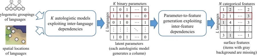
Figure 1: Overview of the proposed Bayesian generative model. Dotted boxes indicate the latent and surface representations of a language. Solid arrows show the direction of stochastic generation.
modeling uncertainties. We demonstrate that we can jointly infer missing values and latent repre-sentations.
Another question left unanswered is how good the induced representations are. In this paper, we present two quantitative analyses of the induced representations. The first one is rather indirect: we measure how well a model recovers missing val-ues, with the assumption that good representations must capture regularity in surface features. We show that the proposed method outperformed the pipelined imputation method ofMurawaki(2015) among others.
The second analysis involves geography. It is well known that the values of a surface feature do not distribute randomly in the world but reflect vertical (phylogenetic) transmissions from parents to children and horizontal (spatial or areal) trans-missions between populations (Nichols, 1992). For example, languages of Mainland Southeast Asia are known for having similar tone systems even though they belong to different language families. To measure the degrees of the two modes of transmissions, we use an autologistic model that investigates dependencies among lan-guages (Towner et al., 2012;Yamauchi and Mu-rawaki, 2016). Since it requires the input to be discrete, we evaluate a new model that fo-cuses on inter-feature dependencies in the same way as Murawaki (2015) but induces binary la-tent representations. We show that vertical and horizontal signals observed for surface features largely vanish from latent representations when only inter-feature dependencies are exploited. Al-though not directly applicable to the model of Mu-rawaki(2015), our results suggest that the pipeline approach suffers from noise during phylogenetic inference. To address this problem, we extend the induction model to incorporate the autologistic model at the level of latent representations, rather
than surface features. With this integrated model, we manage to let induced representations retain surface signals.
In the end, the Bayesian generative model we propose induces binary latent representations by combining feature dependencies and inter-language dependencies, with primacy given to the former (Figure 1). Whereas inter-feature depen-dencies are synchronic in nature, inter-language dependencies reflect diachrony. Thus we call the integrated model diachrony-aware induction.
Due to space limitation, we had to put technical details into the supplementary material. However, we would like to stress that the proposed model works only if it is armed with statistical techniques rarely found in the NLP literature. Together with missing values and binary representations, a large number of continuous variables that connect bi-nary representations to surface features need to be inferred. Unfortunately, a na¨ıve Metropolis-Hastings algorithm does not converge within real-istic time scales. We solve this problem by adopt-ing Hamiltonian Monte Carlo (Neal, 2011) since it enables us to efficiently sample a large num-ber of continuous variables at once. Likewise, the autologistic model contains an intractable normal-ization term, which prevents the application of the standard Metropolis-Hastings sampler. We use an approximate sampler instead (Liang,2010). 2 Related Work
2.1 Inter-feature Dependencies
interac-tion between features. Although these studies en-tirely focused on surface patterns, they imply the presence of some latent structure behind these sur-face features.
Some generative linguists argue for the ex-istence of binary latent parameters behind sur-face features although they are controversial even among generative linguists (Boeckx, 2014). We borrow the term parameter from generative lin-guistics because the name of feature is reserved for surface variables.
Parameters are part of the principles and pa-rameters (P&P) framework (Chomsky and Las-nik, 1993), where, the structure of a language is explained by (1) a set of universal principles that are common to all languages and (2) a set of parameters whose values vary among languages. Here we skip the former since our focus is on structural variability. According to P&P, if we set specific values to all the parameters, then we obtain a specific language. Each parameter is binary and, in general, sets the values of mul-tiple surface features in a deterministic manner. For example, the head directionality parameter is either head-initial or head-final. If head-initialis chosen, then surface features are set to VO, NA and Prepositions; other-wise the language in question becomesOV,ANand Postpositions(Baker,2002). Baker (2002) discussed a number of parameters such as head directionality, polysynthesis, and topic prominent parameters.
Partly inspired by the P&P framework, we use a sequence of binary variables as the latent rep-resentation of a language. However, there are non-negligible differences between P&P and ours, which are discussed in Section S.2 of the supple-mentary material.
What the structure behind surface features looks like is almost exclusively discussed by generative linguists, but it should be noted that they are not the only group who attempts to explain surface patterns. Roughly speaking, generative linguists are part of the synchronist camp, as contrasted withdiachronists, who consider that at least some patterns observed in surface features arise from common paths of diachronic development (Ander-son,2016). An important factor of diachronic de-velopment is grammaticalization, by which con-tent words change into function words (Heine and Kuteva, 2007). For example, the correlation
be-tween the order of adposition and noun and the order of genitive and noun might be explained by the fact that adpositions often derive from nouns.
2.2 Inter-language Dependencies
The standard model for phylogenetic inference is the tree model, where a trait is passed on from a parent to a child with occasional modifications. In fact, the recent success in the applications of statistical models to historical linguistic problems is largely attributed to the tree model (Gray and Atkinson, 2003; Bouckaert et al., 2012). In lin-guistic typology, however, a non-tree-like mode of evolution has emerged as one of the central top-ics (Trubetzkoy, 1928; Campbell, 2006). Typo-logical features, like loanwords, can be borrowed from one language to another, and as a result, ver-tical (phylogenetic) signals are obscured by hori-zontal (spatial) transmission.
The task of incorporating both vertical and hor-izontal transmissions within a statistical model of evolution is notoriously challenging because of the excessive flexibility of horizontal transmissions. This is the reason why previously proposed mod-els are coupled with some very strong assump-tions, for example, that a reference tree is given a priori (Nelson-Sathi et al.,2010), and that horizon-tal transmissions can be modeled through time-invariant areal clusters (Daum´e III,2009).
3 Data and Preprocessing
The dataset we used in the present study is the online edition2 of the World Atlas of Language Structures (WALS) (Haspelmath et al., 2005). While Greenberg(1963) and generative linguists have manually induced patterns and parameters, WALS makes it possible to take computational approaches to modeling features (Daum´e III and Campbell, 2007; Daum´e III, 2009; Murawaki, 2015;Takamura et al.,2016;Murawaki,2016).
WALS is essentially a matrix where languages are represented as rows and features as columns. As of 2017, it contained 2,679 languages and 192 surface features. It covered less than 15% of items in the matrix, however.
We removed sign languages, pidgins and cre-oles from the matrix. We imputed some missing values that could trivially be inferred from other features. We then removed features that covered less than 10% of the languages. After the pre-processing, the number of languagesLwas 2,607 while the number of features N was reduced to 104. The coverage went up to 26.9%, but the rate was still alarmingly low.
In WALS, languages are accompanied by addi-tional information. We used the following fields to model inter-language dependencies. (1) gen-era, the lower of the two-level phylogenetic group-ings, and (2) single-point geographical coordi-nates (longitude and latitude). By connecting ev-ery pair of languages within a genus, we con-structed a phylogenetic neighbor graph. A spatial neighbor graph was constructed by linking all lan-guage pairs that were located within a distance of
R = 1000km. On average, each language had
30.8and89.1neighbors, respectively.
The features in WALS are categorical. For example, Feature 81A, “Order of Subject, Ob-ject and Verb” has seven possible values: SOV, SVO, VSO, VOS, OVS, OSVandNo dominant order, and each language incorporates one of these seven values. For each language, we ar-ranged its features into a sequence. A sequence of categorical features can alternatively be repre-sented as a binary sequence using the 1-of-Fi
cod-ing scheme: FeatureiwithFipossible values was
converted intoFibinary items among which only
one item takes1. The number of binarized features M was 723.
2http://wals.info/
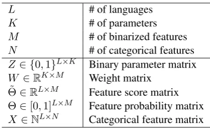
L # of languages
K # of parameters
M # of binarized features N # of categorical features Z ∈ {0,1}L×K Binary parameter matrix
W ∈RK×M Weight matrix
˜Θ∈RL×M Feature score matrix
Θ∈[0,1]L×M Feature probability matrix
X ∈NL×N Categorical feature matrix
Table 1: Notations.
4 Proposed Method
Since the proposed model is rather complicated, we present two key components before going into the integrated model. Table 1 shows notations used in this paper. Surface features have two ways of indexing. First, feature values are serialized as
(1,1),· · ·,(1, F1),(2,1),· · ·,(i, j),· · ·,(N, FN),
where(i, j)points to featurei’sj-th value. Then they are given the flat index 1,· · · , m,· · ·, M (M =PNi=1Fi). Two indices are mapped by the
function f(i, j) = m. We need the flat repre-sentation because that is what latent parameters work on. A parameter is expected to capture the relation between one feature’s particular value (e.g., VO for the order of object and verb) and another feature’s particular value (NAfor the order of adjective and noun).
4.1 Inter-feature Dependencies
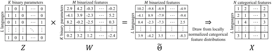
Figure2illustrates how surface features are gen-erated from binary latent parameters. We use ma-trix factorization (Srebro et al.,2005;Griffiths and Ghahramani,2011) to capture inter-feature depen-dencies. Since categorical feature matrixX can-not directly be decomposed into two, we first con-struct (unnormalized) feature score matrix ˜Θ and then stochastically generateXusing ˜Θ.
˜Θis a product of binary parameter matrixZand weight matrixW. The generation ofZwill be de-scribed in Section4.2.3 Each item of ˜Θ,θ˜l,m, is a
score for languagel’sm-th binarized feature. It is affected only by parameters withzl,k = 1because
˜
θl,m= K X
k=1
zl,kwk,m. (1)
3 Although the natural choice for modeling binary
…
Figure 2: Stochastic parameter-to-feature generation. ˜Θ =ZW encodes inter-feature dependencies.
We locally apply normalization to ˜Θ to obtain
Θ, in whichθl,i,j is the probability of language l
taking valuejfor categorical featurei
θl,i,j = Pexp(˜θl,f(i,j))
j0exp(˜θl,f(i,j0)). (2)
Finally, languagel’s i-th categorical feature,xl,i,
is generated from this distribution.
P(xl,i|zl,∗, W) =θl,i,xl,i, (3)
wherezl,∗= (zl,1,· · ·, zl,K).
Combining Eqs. (1) and (2), we obtain
θl,i,j ∝ exp(
We can see from Eq. (4) that this is a product-of-experts model (Hinton, 2002). If zl,k =
0, parameter k has no effect on θl,i,j because
exp(zl,kwk,f(i,j)) = 1. Otherwise, ifwk,f(i,j) > 0, it makesθl,i,jlarger, and ifwk,f(i,j)<0, it
low-ersθl,i,j.
Suppose that for parameter k, a certain group of languages takes zl,k = 1. If two categorical
feature values (i1, j1) and (i2, j2) have positive
weights (i.e.,wk,f(i1,j1) >0andwk,f(i2,j2) > 0), the pair must often co-occur in these languages. Likewise, the fact that two feature values do not co-occur can be encoded as a positive weight for one value and a negative weight for the other.
4.2 Inter-language Dependencies
The autologistic model is used to generate each column of Z, z∗,k = (z1,k,· · · , zL,k). To
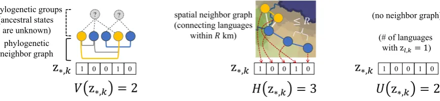
con-struct the model, we use two neighbor graphs and the corresponding three counting functions, as il-lustrated in Figure3. V(z∗,k)returns the number
of pairs sharing the same value in the phylogenetic neighbor graph, andH(z∗,k)is the spatial
equiva-lent ofV(z∗,k). U(z∗,k)gives the number of
lan-guages that take the value1.
We now introduce the following variables: ver-tical stabilityvk >0, horizontal diffusibilityhk >
0, and universality−∞ < uk < ∞for each
fea-turek. Then the probability ofz∗.kconditioned on
vk,hkandukis given as
The denominator is a normalization term, ensuring that the sum of the distribution equals one.
The autologistic model can be interpreted in terms of the competition associated with possible assignments ofz∗,k for the probability mass 1. If
a given value,z∗,k, has a relatively largeV(z∗,k),
then setting a large value forvkenables it to
appro-priate fractions of the mass from its weaker rivals. However, if too large a value is set forvk, then it
will be overwhelmed by its stronger rivals. To acquire further insights into the model, let us consider the probability of language l taking value b ∈ {0,1}, conditioned on the rest of the languages,z−l,k:
P(zl,k =b|z−l,k, vk, hk, uk)∝
exp (vkVl,k,b+hkHl,k,b+ukb), (5)
where Vl,k,b is the number of language l’s
phy-logenetic neighbors that assume value b, and Hl,k,b is its spatial counterpart. P(zl,k = b |
z−l,k, vk, hk, uk)is expressed by the weighted
phy-1 0 0 phy-1
z
∗,𝑘𝑘 0? ?
phylogenetic groups (ancestral states
are unknown) phylogenetic neighbor graph
𝑉𝑉
z
∗,𝑘𝑘= 2
𝐻𝐻
z
∗,𝑘𝑘= 3
spatial neighbor graph (connecting languages
within 𝑅𝑅km)
≤ 𝑅𝑅
1 0 0 1
z
∗,𝑘𝑘 0𝑈𝑈
z
∗,𝑘𝑘= 2
1 0 0 1z
∗,𝑘𝑘 0(# of languages with z𝑙𝑙,𝑘𝑘= 1)
(no neighbor graph)
Figure 3: Neighbor graphs and counting functions used to encode inter-language dependencies.
logenetic neighbors of languagel, but it also de-pends on its spatial neighbors and on universality. How strongly these factors affect the stochastic se-lection is controlled byvk,hk, anduk.
4.3 Integrated Model
Now we complete the generative model by inte-grating the two types of dependencies. The joint distribution is defined as
P(A, Z, W, X)=P(A)P(Z|A)P(W)P(X|Z, W),
where hyperparameters are omitted for brevity and Ais a set of latent variables that control the gener-ation ofZ:
P(A) =YK
k=1
P(vk)P(hk)P(uk).
Their prior distributions are:vk ∼Gamma(κ, θ),
hk ∼Gamma(κ, θ), anduk∼ N(0, σ2).4
Next, z∗,k’s are generated as described in
Sec-tion4.2:
P(Z |A) =YK
k=1
P(z∗,k |vk, hk, uk).
The generation of Z is followed by that of the corresponding weight matrix W ∈ RK×M, and
then we obtain the feature score matrix ˜Θ =ZW. Each item of W, wk,m, is generated from
Stu-dent’st-distribution with 1 degree of freedom. We choose this distribution for two reasons. First, it has heavier tails than the Gaussian distribution and allows some weights to fall far from 0. Sec-ond, our inference algorithm demands that the negative logarithm of the probability density func-tion be differentiable (see Secfunc-tion S.4 for details).
4 In the experiments, we set shapeκ = 1, scaleθ = 1,
and standard deviationσ= 10. These priors were not non-informative, but they were sufficiently gentle in the regions where these parameters typically resided.
Thet-distribution satisfies the condition while the Laplace distribution does not.
Finally,X is generated using ˜Θ =ZW, as de-scribed in Section4.1:
P(X|Z, W) =YL
l=1 N Y
i=1
P(xl,i|zl,∗, W).
4.4 Inference
As usual, we use Gibbs sampling to perform pos-terior inference. Given observed values xl,i, we
iteratively updatezl,k,vk,hk,uk, andwk,∗as well as missing valuesxl,i.
Updatexl,i. xl,iis sampled from Eq. (3).
Update zl,k. The posterior probability
P(zl,k| −) is proportional to Eq. (5) times
the product of Eq. (3) for all feature i’s of languagel.
Update vk, hk and uk. We want to sample vk
(andhkanduk) fromP(vk| −)∝P(vk)P(z∗,k |
vk, hk, uk). This belongs to a class of problems
known as sampling from doubly-intractable distri-butions (Møller et al.,2006;Murray et al.,2006). While it remains a challenging problem in statis-tics, it is not difficult to approximately sample the variables if we give up theoretical rigorous-ness (Liang, 2010). The details of the algorithm we use can be found in Section S.3 of the supple-mentary material.
Updatewk,∗. The remaining problem is how to updatewk,m. Since the number of weights is very
large (K ×M), the simple Metropolis-Hastings algorithm (G¨or¨ur et al.,2006;Doyle et al.,2014) is not a workable option. To address this problem, we block-samplewk,∗ = (wk,1,· · ·, wk,M)using
5 Experiments
5.1 Missing Value Imputation
We indirectly evaluated the proposed model, called SYNDIA, by means of missing value im-putation. If it predicts missing feature values bet-ter than reasonable baselines, we can say that the induced parameters are justified. Although no ground truth exists for the missing portion of the dataset, missing value imputation can be evaluated by hiding some observed values and verifying the effectiveness of their recovery. We conducted a 10-fold cross-validation.
We ran SYNDIA with two different settings: K = 50and100. We performed posterior infer-ence for 500 iterations. After that, we collected 100 samples ofxl,ifor each language, one per
it-eration. For each missing valuexl,i, we output the
most frequent value among the 100 samples. The HMC parametersandSwere set to0.05and10, respectively.
We applied simulated annealing to the sampling ofzl,k. For the first 100 iterations, the inverse
tem-perature was increased from0.1to1.0.
We compared SYNDIAwith several baselines.
MFV For each categorical featurei, always out-put the most frequent value among observedxl,i.
Surface-DIA An autologistic model applied to
surface features (Yamauchi and Murawaki, 2016). The details of the model are presented in Section S.5 of the supplementary material.
DPMPM A Dirichlet process mixture of multino-mial distributions with a truncated stick-breaking construction (Si and Reiter,2013) used byBlasi et al.(2017). It assigns a single categorical latent variable to each language. As an implementa-tion, we used theRpackageNPBayesImpute.
MCA A variant of multiple correspondence anal-ysis (Josse et al., 2012) used by Murawaki (2015). We used the imputeMCA function of theRpackagemissMDA.
SYN A simplified version of SYNDIA, with vk andhkremoved from the model. See Section S.6
of the supplementary material for details. MFV and Surface-DIAcan be seen as the models of inter-language dependencies while DPMPM, MCA and SYN are these of inter-feature depen-dencies.
Table 2 shows the result. We can see that SYNDIA with K = 50 performed the best.
Type Model Accuracy
Lang. MFVSurface-DIA 60.95%66.22%
Feat.
DPMPM (K∗ = 50) 69.08%
MCA 69.88%
SYN(K= 50) 73.83%
SYN(K= 100) 72.87%
Both SSYNYNDDIAIA(K(K= 100= 50)) 74.00%74.46%
Table 2: Accuracy of missing value imputation. The first column indicates the types of cies the models exploit: inter-language dependen-cies, inter-feature dependencies and both.
Model Accuracy
Full model (SYNDIA) 74.46%
-vertical 73.89%
-horizontal 74.47%
-vertical -horizontal (SYN) 73.83% Table 3: Ablation experiments for missing value imputation.K = 50.
Smaller K yielded higher accuracy although the likelihoodP(X |Z, W)went up asKincreased. Due to the high ratio of missing values, the model might have overfitted the data with largerK.
The fact that SYN outperformed Surface-DIA suggests that inter-feature dependencies have more predictive power than inter-language depen-dencies in the dataset. However, they are compli-mentary in nature as SYNDIAoutperformed SYN. We can confirm the limited expressive power of single categorical latent variables because DPMPM performed poorly even if a small value was set to the truncation level K∗ to avoid over-fitting. MCA employs more expressive represen-tations of a sequence of continuous variables for each language. It slightly outperformed DPMPM but was beaten by SYNby a large margin. We con-jecture that MCA was more sensitive to initializa-tion than the Bayesian model armed with MCMC sampling. In any case, this result indicates that the latent representations Murawaki (2015) obtained were of poorer quality than those of SYN, not to mention those of SYNDIA.
We also conducted ablation experiments by re-moving eithervkorhkfrom the model. The result
0.000 0.005 0.010 0.015 0.020 0.025 0.030
Horizontal diffusibilityhi
0.00 0.01 0.02 0.03 0.04 0.05 0.06
V
ertical
stability
vi
Feature: Phonology Feature: Morphology Feature: Nominal Categories Feature: Nominal Syntax Feature: Verbal Categories Feature: Word Order Feature: Simple Clause Feature: Complex Sentences Feature: Lexicon
Parameter (SYNDIA)
0.000 0.005 0.010 0.015 0.020 0.025 0.030
Horizontal diffusibilityhi
0.00 0.01 0.02 0.03 0.04 0.05 0.06
V
ertical
stability
vi
Feature: Phonology Feature: Morphology Feature: Nominal Categories Feature: Nominal Syntax Feature: Verbal Categories Feature: Word Order Feature: Simple Clause Feature: Complex Sentences Feature: Lexicon
Parameter (SYN)
Figure 4: Scatter plots of surface features and induced parameters, with vertical stabilityvi (vk) as the
y-axis and horizontal diffusibilityhi (hk) as the x-axis. Larger vi (hi) indicates that feature iis more
stable (diffusible). Comparing the absolute values of aviand anhimakes no sense because they are tied
with different neighbor graphs. Features are classified into 9 broad categories (calledAreain WALS).vk
(andhk) is the geometric mean of the 100 samples. The induction models are SYNDIA(Top) and SYN
(Bottom). For both models,K = 50.
5.2 Vertical and Horizontal Signals
Hereafter we use all observed features to perform posterior inference. We examined how vertically stable and horizontally diffusible the induced pa-rameters were. For SYNDIA, we simply extracted vk andhk from posterior samples. For
compari-son, we used Surface-DIAto estimate vertical sta-bility and horizontal diffusista-bility of surface fea-tures. The same autologistic model was used to estimatevk andhk of SYNafterthe posterior
in-ference. For details, see Sections S.5 and S.6.2 of the supplementary material.
Figure 4 summarizes the results. We can see that the most vertically stable latent parameters of SYNDIAare comparable to the most vertically sta-ble surface features. The same holds for the most horizontally diffusible ones. Thus we can con-clude that the induced representations retain
ver-tical and horizontal signals observed for surface features.
On the other hand, SYNhalved vertical stabil-ity and horizontal diffusibilstabil-ity when transform-ing surface features into latent parameters. A plausible explanation of this failure is that for many scarcely documented languages, we sim-ply did not have enough observed surface fea-tures to determine their latent representations only from inter-feature dependencies. Due to the in-herent uncertainty, zl,k swung between 0 and 1
during posterior inference, regardless of the states of their neighbors. As a result, these languages seem to have blocked vertical and horizontal sig-nals. By contrast, SYNDIAappears to have flipped zl,k without disrupting inter-language
dependen-cies when there were.
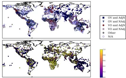
neg-OV and AdjN OV and NAdj VO and AdjN VO and NAdj Other N/A
0.0 0.2 0.4 0.6 0.8 1.0
Figure 5: A comparison of a surface feature and a latent parameter in terms of geographical distribution. Each point denotes a language. (Top) Feature 97A, “Relationship between the Order of Object and Verb and the Order of Adjective and Noun.” Missing values are denoted asN/A. (Bottom) A parameter of SYNDIAwithK0= 50. Lighter nodes indicate higher frequencies ofzl,k = 1among 100 samples.
ative implications for the pipeline approach pur-sued byMurawaki(2015), where the inter-feature dependency-based induction of latent representa-tions is followed by phylogenetic inference. For-tunately, evidence presented up to this point sug-gests that it can be readily replaced with the pro-posed model.
5.3 Discussion
Figure5compares a latent parameter of SYNDIA with a surface feature on the world map. Some surface features show several geographic clusters of large size, telling something about the evolu-tionary history of languages. Even with a large number of missing values, SYNDIAyielded com-parable geographic clusters for some parameters. Some geographic clusters were also produced by SYN, especially when the estimation of zl,k was stable. In our subjective evaluation, SYNDIA ap-peared to show clearer patterns than SYN. Need-less to say, not all surface features were associated with clear geographic patterns, and not all latent parameters were. Overall, the results shed a posi-tive light on the applicability of the induced repre-sentations to phylogenetic inference.
We also checked the weight matrix W
(Fig-ure S.2). It is not easy to analyze qualitatively but it deserves future investigation.
6 Conclusion
In this paper, we presented a Bayesian model that induces binary latent parameters from sur-face features of linguistic typology. We combined inter-language dependencies with inter-feature de-pendencies to obtain the latent representations of better quality. Gathering various statisti-cal techniques, we managed to create the com-plex but workable model. The source code is publicly available at https://github.com/ murawaki/latent-typology.
We pointed out that typology-based phyloge-netic inference proposed by Murawaki (2015) had weak foundations, and we rebuilt them from scratch. The whole long paper was needed to do so, but our ultimate goal is the same as the one stated by Murawaki (2015). In the future, we would like to utilize the new latent representations to uncover the evolutionary history of languages. Acknowledgments
References
Stephen R. Anderson. 2016. Synchronic versus
di-achronic explanation and the nature of the language
faculty.Annual Review of Linguistics, 2:1–425.
Mark C. Baker. 2002. The Atoms of Language: The
Mind’s Hidden Rules of Grammar. Basic Books.
Julian Besag. 1974. Spatial interaction and the statisti-cal analysis of lattice systems. Journal of the Royal Statistical Society. Series B (Methodological), pages 192–236.
Dami´an E. Blasi, Susanne Maria Michaelis, and Martin
Haspelmath. 2017. Grammars are robustly
transmit-ted even during the emergence of creole languages.
Nature Human Behaviour.
Cedric Boeckx. 2014. What principles and
parame-ters got wrong. In M. Carme Picallo, editor,
Tree-banks: Building and Using Parsed Corpora, pages 155–178. Oxford University Press.
Remco Bouckaert, Philippe Lemey, Michael Dunn, Simon J. Greenhill, Alexander V. Alekseyenko, Alexei J. Drummond, Russell D. Gray, Marc A.
Suchard, and Quentin D. Atkinson. 2012. Mapping
the origins and expansion of the Indo-European
lan-guage family.Science, 337(6097):957–960.
Lyle Campbell. 2006. Areal linguistics. In
Encyclo-pedia of Language and Linguistics, Second Edition, pages 454–460. Elsevier.
Noam Chomsky and Howard Lasnik. 1993. The the-ory of principles and parameters. In Joachim Ja-cobs, Arnim von Stechow, Wolfgang Sternefeld, and
Theo Vennemann, editors,Syntax: An International
Handbook of Contemporary Research, volume 1, pages 506–569. De Gruyter.
Hal Daum´e III. 2009. Non-parametric Bayesian areal
linguistics. In Proceedings of Human Language
Technologies: The 2009 Annual Conference of the North American Chapter of the Association for Computational Linguistics, pages 593–601.
Hal Daum´e III and Lyle Campbell. 2007. A Bayesian model for discovering typological implications. In Proceedings of the 45th Annual Meeting of the Asso-ciation of Computational Linguistics, pages 65–72.
Gabriel Doyle, Klinton Bicknell, and Roger Levy.
2014. Nonparametric learning of phonological
con-straints in optimality theory. InProceedings of the
52nd Annual Meeting of the Association for Compu-tational Linguistics (Volume 1: Long Papers), pages 1094–1103.
Dilan G¨or¨ur, Frank J¨akel, and Carl Edward Rasmussen. 2006. A choice model with infinitely many latent
features. In Proceedings of the 23rd International
Conference on Machine Learning, pages 361–368.
Russell D. Gray and Quentin D. Atkinson. 2003. Language-tree divergence times support the
Ana-tolian theory of Indo-European origin. Nature,
426(6965):435–439.
Joseph H. Greenberg, editor. 1963. Universals of lan-guage. MIT Press.
Thomas L. Griffiths and Zoubin Ghahramani. 2011. The Indian buffet process: An introduction and
review. Journal of Machine Learning Research,
12:1185–1224.
Martin Haspelmath, Matthew Dryer, David Gil, and
Bernard Comrie, editors. 2005. The World Atlas of
Language Structures. Oxford University Press.
Bernd Heine and Tania Kuteva. 2007. The Genesis
of Grammar: A Reconstruction. Oxford University Press.
Geoffrey E. Hinton. 2002.Training products of experts
by minimizing contrastive divergence.Neural
Com-putation, 14(8):1771–1800.
Yoshiaki Itoh and Sumie Ueda. 2004. The ising
model for changes in word ordering rules in
natu-ral languages. Physica D: Nonlinear Phenomena,
198(3):333–339.
Julie Josse, Marie Chavent, Benot Liquet, and Franc¸ois
Husson. 2012. Handling missing values with
reg-ularized iterative multiple correspondence analysis.
Journal of Classification, 29(1):91–116.
Faming Liang. 2010. A double Metropolis–Hastings
sampler for spatial models with intractable
normal-izing constants. Journal of Statistical Computation
and Simulation, 80(9):1007–1022.
Jesper Møller, Anthony N. Pettitt, R. Reeves, and
Kasper K. Berthelsen. 2006. An efficient Markov
chain Monte Carlo method for distributions with
intractable normalising constants. Biometrika,
93(2):451–458.
Yugo Murawaki. 2015. Continuous space
representa-tions of linguistic typology and their application to
phylogenetic inference. InProceedings of the 2015
Conference of the North American Chapter of the Association for Computational Linguistics: Human Language Technologies, pages 324–334.
Yugo Murawaki. 2016. Statistical modeling of creole
genesis. InProceedings of the 2016 Conference of
the North American Chapter of the Association for Computational Linguistics: Human Language Tech-nologies.
Iain Murray, Zoubin Ghahramani, and David J. C. MacKay. 2006. MCMC for doubly-intractable
dis-tributions. In Proceedings of the Twenty-Second
Radford M. Neal. 2011. MCMC using Hamilto-nian dynamics. In Steve Brooks, Andrew Gelman,
Galin L. Jones, and Xiao-Li Meng, editors,
Hand-book of Markov Chain Monte Carlo, pages 113–162. CRC Press.
Shijulal Nelson-Sathi, Johann-Mattis List, Hans Geisler, Heiner Fangerau, Russell D. Gray, William
Martin, and Tal Dagan. 2010. Networks uncover
hidden lexical borrowing in Indo-European
lan-guage evolution. Proceedings of the Royal Society
B: Biological Sciences.
Johanna Nichols. 1992. Linguistic Diversity in Space
and Time. University of Chicago Press.
Johanna Nichols. 1994. The spread of language around
the Pacific rim. Evolutionary Anthropology: Issues,
News, and Reviews, 3(6):206–215.
Johanna Nichols. 1995. Diachronically stable struc-tural features. In Henning Andersen, editor, Histor-ical Linguistics 1993. Selected Papers from the 11th International Conference on Historical Linguistics, Los Angeles 16–20 August 1993. John Benjamins Publishing Company.
Mikael Parkvall. 2008. Which parts of language are the
most stable? STUF-Language Typology and
Uni-versals Sprachtypologie und Universalienforschung, 61(3):234–250.
Yajuan Si and Jerome P. Reiter. 2013. Nonparametric
Bayesian multiple imputation for incomplete
cate-gorical variables in large-scale assessment surveys.
Journal of Educational and Behavioral Statistics, 38(5):499–521.
Nathan Srebro, Jason D. M. Rennie, and Tommi S. Jaakkola. 2005. Maximum-margin matrix factoriza-tion. InProceedings of the 17th International Con-ference on Neural Information Processing Systems, pages 1329–1336.
Hiroya Takamura, Ryo Nagata, and Yoshifumi Kawasaki. 2016. Discriminative analysis of linguis-tic features for typological study. InProceedings of the Tenth International Conference on Language Re-sources and Evaluation (LREC 2016), pages 69–76.
Mary C. Towner, Mark N. Grote, Jay Venti, and
Monique Borgerhoff Mulder. 2012. Cultural
macroevolution on neighbor graphs: Vertical and horizontal transmission among western north
Amer-ican Indian societies. Human Nature, 23(3):283–
305.
Nikolai Sergeevich Trubetzkoy. 1928. Proposition 16. In Acts of the First International Congress of Lin-guists, pages 17–18.
Søren Wichmann and Eric W. Holman. 2009. Temporal
Stability of Linguistic Typological Features. Lincom Europa.
Kenji Yamauchi and Yugo Murawaki. 2016. Contrast-ing vertical and horizontal transmission of
typolog-ical features. In Proceedings of COLING 2016,