Exploring the Use of Word Relation Features
for Sentiment Classification
Rui Xia and Chengqing Zong
National Laboratory of Pattern Recognition
Institute of Automation, Chinese Academy of Sciences
{rxia, cqzong}@nlpr.ia.ac.cn
Abstract
Word relation features, which encode relation information between words, are supposed to be effective features for sentiment classification. However, the use of word relation features suffers from two issues. One is the sparse-data problem and the lack of generalization performance; the other is the limitation of using word relations as additional features to unigrams. To address the two issues, we propose a generalized word relation feature extraction method and an ensemble model to efficiently inte-grate unigrams and different type of word relation features. Furthermore, aimed at reducing the computation complexity, we propose two fast feature selection methods that are specially de-signed for word relation features. A range of experiments are conducted to evaluate the effectiveness and efficiency of our approaches.
1
Introduction
The task of text sentiment classification has be-come a hotspot in the field of natural language processing in recent years (Pang and Lee, 2008). The dominating text representation method in sentiment classification is known as the bag-of-words (BOW) model. Although BOW is quite simple and efficient, a great deal of the informa-tion from original text is discarded, word order is disrupted and syntactic structures are broken. Therefore, more sophisticated features with a deeper understanding of the text are required for sentiment classification tasks.
With the attempt to capture the word relation information behind the text, word relation (WR) features, such as higher-order n-grams and word dependency relations, have been employed in text representation for sentiment classification (Dave et al., 2003; Gamon, 2004; Joshi and Penstein-Rosé, 2009).
However, in most of the literature, the per-formance of individual WR feature set was poor, even inferior to the traditional unigrams. For this reason, WR features were commonly used as additional features to supplement unigrams, to encode more word order and word relation information. Even so, the performance of joint features was still far from satisfactory (Dave et al., 2003; Gamon, 2004; Joshi and Penstein-Rosé, 2009).
We speculate that the poor performance is possibly due to the following two reasons: 1) in WR features, the data are sparse and the fea-tures lack generalization capability; 2) the use of joint features of unigrams and WR features has its limitation.
On one hand, there were attempts at finding better generalized WR (GWR) features. Gamon (2004) back off words in n-grams (and semantic relations) to their respective POS tags (e.g.,
great-movie to adjective-noun); Joshi and Rosé (2009) propose a method by only backing off the head word in dependency relation pairs to its POS tag (e.g., great-movie to great-noun), which are supposed to be more generalized than word pairs. Based on Joshi and Rosé’s method, we back off the word in each word relation pairs to its corresponding POS cluster, making the feature space smarter and more effective.
in-creased. Although the discriminative model (e.g., SVM) is proven to be more effective on unigrams (Pang et al., 2002) for its ability of capturing the complexity of more relevant fea-tures, WR features are more inclined to work better in the generative model (e.g., NB) since the feature independence assumption holds well in this case.
Based on this finding, we therefore intuitively seek, instead of jointly using unigrams and GWR features, to efficiently integrate them to synthesize a more accurate classification proce-dure. We use the ensemble model to fuse differ-ent types of features under distinct classification models, with an attempt to overcome individual drawbacks and benefit from each other’s merit, and finally to enhance the overall performance.
Furthermore, feature reduction is another im-portant issue of using WR features. Due to the huge dimension of WR feature space, traditional feature selection methods in text classification perform inefficiently. However, to our knowl-edge, no related work has focused on feature selection specially designed for WR features.
Taking this point into consideration, we pro-pose two fast feature selection methods (FMI and FIG) for GWR features with a theoretical proof. FMI and FIG regard the importance of a GWR feature as two component parts, and take the sum of two scores as the final score. FMI and FIG remain a close approximation to MI and IG, but speed up the computation by at most 10 times. Finally, we apply FMI and FIG to the ensemble model, reducing the computation complexity to a great extent.
The remainder of this paper is organized as follows. In Section 2, we introduce the approach to extracting GWR features. In Section 3, we present the ensemble model for integrating dif-ferent types of features. In Section 4, the fast feature selection methods for WR features are proposed. Experimental results are reported in Section 5. Section 6 draws conclusions and out-lines directions for future work.
2
Generalized Word Relation Features
A straightforward method for extracting WR features is to simply map word pairs into the feature vector. However, due to the sparse-data problem and the lack of generalization ability, the performance of WR is discounted. Consider the following two pieces of text:
1) Avatar is a great movie. I definitely rec-ommend it.
2) I definitely recommend this book. It is great.
We lay the emphasis on the following word pairs: great-movie, great-it, it-recommend, and
book-recommend. Although these features are good indicators of sentiment, due to the sparse-data problem, they may not contribute as impor-tantly as we have expected in machine learning algorithms. Moreover, the effects of those fea-tures would be greatly reduced when they are not captured in the test dataset (for example, a new feature great-song in the test set would never benefit from great-movie and great-it).
Joshi and Rosé (2009) back off the head word in each of the relation pairs to its POS tag. Tak-ing great-movie for example, the back-off fea-ture will be great-noun. With such a transforma-tion, original features like great-movie, great-book and other great-noun pairs are regarded as one feature, hence, the learning algorithms could learn a weight for a more general feature that has stronger evidence of association with the class, and any new test sentence that con-tains an unseen noun in a similar relationship with the adjective great (e.g., great-song) will receive some weight in favor of the class label.
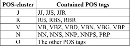
With the attempt to make a further generali-zation, we conduct a POS clustering. Consider-ing the effect of different POS tags in both uni-grams and word relations, the POS tags are categorized as shown in Table 1.
POS-cluster Contained POS tags
J JJ, JJS, JJR
R RB, RBS, RBR
V VB, VBZ, VBD, VBN, VBG, VBP
N NN, NNS, NNP, NNPS, PRP
O The other POS tags
Table 1: POS Clustering (the Penn Corpus Style)
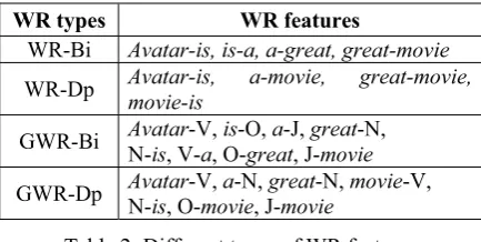
Taking “Avatar is a great movie” for example, different types of WR features are presented in Table 2, where Uni denotes unigrams; WR-Bi indicates traditional bigrams; WR-Dp indicates word pairs of dependency relation; GWR-Bi and GWR-Dp respectively denote generalized bigrams and dependency relations.
WR types WR features
WR-Bi Avatar-is, is-a, a-great, great-movie
WR-Dp Avatar-is, a-movie, great-movie,
movie-is
GWR-Bi Avatar-V, is-O, a-J, great-N, N-is, V-a, O-great, J-movie
GWR-Dp Avatar-V, a-N, great-N, movie-V,
N-is, O-movie, J-movie
Table 2: Different types of WR features
3
An Ensemble Model for Integrating
WR Features
3.1 Joint Features, Good Enough?
Although the unigram feature space is simple, and the WR features are more sophisticated, the latter was mostly used as extra features in addi-tion to the former, rather than to substitute it. Even so, in most of the literature, the improve-ments of joint features are still not as good as we had expected. For example, Dave et al. (2003) try to extract a refined subset of WR pairs (adjective-noun, subject-verb, and verb-object pairs) as additional features to traditional unigrams, but do not get significant improve-ments. In the experiments of Joshi and Rosé (2009), the improvements of unigrams together with WR features (even generalized WR features) are also not remarkable (sometimes even worse) compared to simple unigrams.
One possible explanation might be that dif-ferent types of features have distinct distribu-tions, and therefore would probably yield vary performance on different machine learning al-gorithms. For example, the generative model is optimal if the distribution is well estimated; otherwise the performance will drop signifi-cantly (for instance, NB performs poorly unless the feature independence assumption holds well). While on the contrary, the discriminative model such as SVM is good at representing the complexity of relevant features.
Let us review the results reported by Pang and Lee (2002) that compare different classifi-cation algorithms: SVM performs significantly
better than NB on unigrams; while the outcome is the opposite on bigrams. It is possibly due to that from unigrams to bigrams, the relevance between features is reduced (bigrams cover some relevance of unigram pairs), and the inde-pendence between features increases.
Since GWR features are less relevant and more independent in comparison, it is reason-able for us to infer that these features would work better on NB than on SVM. We therefore intuitively seek to employ the ensemble model for sentiment classification tasks, with an at-tempt to efficiently integrate different types of features under distinct classification models.
3.2 Model Formulation
The ensemble model (Kittler, 1998), which combines the outputs of several base classifiers to form an integrated output, has become an effective classification method for many do-mains.
For our ensemble task, we train six base clas-sifiers (the NB and SVM model respectively on the Uni, GWR-Bi and GWR-Dp features). By mapping the probabilistic outputs (for C classes) of Dbase classifiers into the meta-vector
11 1 1
ˆ[o , oC, ,okj, ,oD, oDC],
x ! ! ! ! (1)
the weighted ensemble is formulized by
1 1
ˆ ˆ
( ) ,
D D
j j k kj k k
k k
O g X o X xq
x
D j (2)where is the weight assigned to the -th ss
mization
, we use descent
defined as k
X k
base cla ifier.
3.3 Weight Opti
Inspired by linear regression
methods to seek optimization according to cer-tain criteria. We employ two criteria, namely the perceptron criterion and the minimum clas-sification error (MCE) criterion.
The perceptron cost function is
1, , 1
1 N
ˆ ˆ
max ( ) ( ) .
i
p j i y i
j C i
J g g
N
¯
¡ °
¢ ±
x x! (3)
The minimization of Jp is approximately equal sc
1992) is
function is given by
1 1
where is the sigmoid function.
For both criteria, stochastic gradient descent . SGD uses ( )
E<
(SGD) is utilized for optimization
approximate gradients estimated from subsets of the training data and updates the parameters in an online manner:
( 1) ( ) ( )
The gradients of perceptron and MCE cost
p
As for perceptron criterion, we employ the average perceptron (AvgP) (Freund and Sc
In the past decade, feature selection (FS) studies n.
pose a fast feature selection method that is specially designed for GWR features. In our method, the
re (e.g.,
great-hapire, 1999), a variation of perceptron model that averages the weights of all iteration loops, to improve the generalization performance.
4
Feature Selection for WR Features
mainly focus on topical text classificatio (Yang and Pedersen, 1997) investigate five FS metrics and reported that good FS methods (such as IG and CHI) can improve the categori-zation accuracy with an aggressive feature re-moval. In sentiment classification tasks, tradi-tional FS methods were also proven to be effec-tive (Ng et al., 2006; Li et al., 2009).
With regard to WR features, since the dimen-sion of feature space has sharply increased, the amount of computation is considerably large when employing traditional FS methods.
4.1 Fast MI and Fast IG
In order to address this problem, we pro
importance of a GWR featu ws
movie) is considered as two component parts: the non-back-off word w (great) and the POS pairs s (J-N). We calculate the score of w and
s respectively using existing FS methods, and take the sum of them as the final score. By as-suming the two parts are mutually independent, the im ortance of a relation feature can be taken separately. We now give a theoretical support.
First, the mutual information between a rela-tion feature ws and class ck is defined as
ula (9) indicates that under the assum tion that two component parts and
Form
p-w s of a relation feature are mutually
the mutual in
ws
formation of the relation feature independent,
( , k)
I ws c equals the sum of two component parts I w c( , k) and I s c( , k).
Since the aver mutual information across all classes ( )
weighted average of Yang an dersen (1997) show that the in-formation gain G t( ) is the
( , k)
I t c and I t c( , k)
can cons
. Therefore, with the sa ider the infor
ula
t IG (FIG) respectively. Now let of the independ-ence assumption. In fact in a rel
tw
me mation gain of reason, we
us look back at the rationality
( )
G ws
con-sider a GWR feature as a combination of the non-back-off word and the POS pairs, the as-sumption will be easier to satisfy. Taking great-movie (great-N) for example, compared to great
and N, great and J-N are more independent (J-N covers some relation information), therefore it is more feasible to take G great( )G(J-N) as an approximation of G great( -N).
Laying aside the assumption, we place em-phasis on the advantage of FIG (FMI) in com-putational efficiency. A ension of the unigrams feature sp
ssuming the dim ace is , and ignor-in
escribed in section 3.2. In
-on
ense
the effective-lection.
, 2004) is used in ment-level polarit positive and 1,000
N
N
g the data-sparse problem, the dimension of the GWR feature space is 2 5q qN (backing off head/modifier word to 5 POS-cluster). Tradi-tional IG (MI) feature selection needs to calcu-late the score of all 10qN features, while FIG (FMI) only needs to comp words and 25 POS pairs. That is to say, FIG (FMI) can speed up the computation of traditional IG (MI) by at most 10 times.
4.2 Integration with the Ensemble Model
We now present how FMI (FIG) is applied to the ensemble model d
ute for
each of the six base-classifiers described in Sec tion 3.2, feature selection is performed (tradi tional IG on unigrams, FIG on GWR features). Note that when performing FIG on individual GWR feature sets, the computation of non-back-off word G w( ), is taken care of by having already computed IG on unigrams. Thus, we
ly need to compute the score of 25 POS pairs. From this point of view, FIG (FMI) is quite suitable for the mble model.
5
Experiments
We first present the performance of system per-formance, and then demonstrate
ness of fast feature se
5.1 Experimental Setup
Datasets: The Cornell movie-review dataset1 introduced by (Pang and Lee
our experiments. It is a docu dataset that contains 1,000
y
negative processed reviews.
1
http://www.cs.cornell.edu/people/pabo/movie-review-data/
We also use the dataset2 introduced in (Joshi and Penstein-Rosé, 2009) for comparison. It is a su
t and the E-product dataset is at
l (McCallum
ts are
d Ženko, 2004) is employed. Ta
e accuracy.
gan- per-bset (200 sentences each for 11 different products) of the product review dataset released by (Hu and Liu, 2004). We will refer to it E-product dataset.
The Movie dataset is a domain-specific docu-ment-level datase
sentence-level and cross-domain. We conduct experiments on both of them to evaluate our approach in a wide range of tasks.
Classifier: We implement the NB classifier based on a multinomial event mode
and Nigam, 1998) with Laplace smoothing. The tool LIBSVM3 is chosen as the SVM classifier. Setting of kernel function is linear kernel, the penalty parameter is set to one, and the Platt’s probabilistic output for SVM is applied to ap-proximate the posterior probabilities. Term presence is used as the feature weighting.
Implementation: The Movie dataset is evenly divided into 5 folds, and all the experimen conducted with a 5-fold cross validation. Fol-lowing the settings by Joshi and Rosé, an 11-fold cross validation is applied to E-product dataset, where each test fold contains all the sentences for one of the 11 products, and the sentences for the remaining 10 products are used for training.
For ensemble learning, the stacking frame-work (Džeroski an
king the Movie dataset for example, in each loop of the 5-fold cross validation, the probabil-istic outputs of the test fold are considered as test samples for ensemble leaning; and an inner 4-fold leave-one-out procedure is applied to the training data, where samples in each fold are trained on the remaining three folds to obtain the probabilistic outputs which serve as training samples for ensemble learning.
All the performance in the remaining tables and figures is in terms of averag
5.2 Results of Classification Accuracy
The results of classification accuracy are or ized in three parts. We first compare the formance of individual WR and GWR; secondly we compare joint features and the ensemble
2
http://www.cs.cmu.edu/~maheshj/datasets/acl09short.html
3
model; thirdly we compare different ensemble strategies; finally we make a comparison with some related work.
5.2.1 WR vs. GWR
Table 3 presents the re feature sets. Four types
sults of individual WR of WR features, includ-ing WR-Bi, WR-Dp, GWR-Bi and GWR-Dp, are examined under two classification models on two datasets. For each of the results, we re-port the best accuracy under feature selection.
Model WR Feature Movie E-product
WR-Bi 83.05 63.27 GWR-Bi 85.55 65.17
WR-Dp 82.15 65.14 SVM
GWR-Dp 83.40 67.09 WR-Bi 84.60 66.86 GWR-Bi 85.45 67.50
WR-Dp 83.90 65.68 NB
GWR-Dp 83.65 67.41
Table 3: Acc ) of I al WR e
Sets
formance of individua R and WR. With the SV
uracies (% ndividu Featur
At first, we place the emphasis on the per-l GW
M model, the performance of GWR features is remarkable compared to traditional WR pairs. Specifically, on the Movie dataset, GWR-Bi outperforms WR-Bi by 2.50%, and GWR-Dp outperforms WR-Dp by 1.35%; on the E-product dataset, the improvements are 1.90% and 1.95%. Under the NB model, on the Movie dataset, GWR-Bi outperforms WR-Bi by 0.85%; on the E-product dataset, GWR-Bi outperforms WR-Bi by 0.64% and GWR-Dp outperforms WR-Dp by 1.73%. One exception is GWR-Dp on the Movie dataset, but the decline is slight (0.25%).
WR Feature Movie E-product
WR-Bi 386k 21k GWR-Bi 152k 16k
WR-Dp 455k 24k GWR-Dp 151k 16k
Table ion of ual Fe Space
fe
-ag
nt in
s
4: Dimen Individ ature
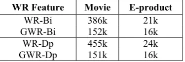
Secondly, we compare the dimensions of dif-rent feature space. Table 4 presents the aver
e size of different types of feature spaces on two datasets. On the Movie dataset, the size of GWR feature space has been significantly re-duced (386k vs. 152k in Bi; 455k vs. 151k in Dp). On the E-product dataset, since the training
set are made up by 10 different domains, data are quite sparse, therefore, the extent of dimen-sion reduction is not as sound as that on Movie dataset, but still considerable (21k vs. 16k in Bi; 24k vs. 16k in Dp).
5.2.2 Joint Features vs. Ensemble Model
The performance of individual feature sets, joi feature set and ensemble model is reported Table 5. Uni, GWR-Bi and GWR-Dp are used as individual features sets in the ensemble model, and Joint Features denote the union of three individual sets. For feature selection, IG is used in Joint Features, and FIG is used in the ensemble model. The reported results are in terms of the best accuracy under feature selec-tion.
Feature and Model Movie E-product
SVM 85.20 67.77 Uni
NB 84.10 66.18 SVM 85.55 65.17 GWR-Bi
NB 85.45 67.50 SVM 83.40 67.09 GWR-Dp
NB 83.65 67.41 SVM 86.10 66.55 Joint Features
NB 85.20 67.64 AvgP 88.60 70.14 E
M nsemble Model
CE 88.55 70.18
Table 5: Accuracies Co t Fe
Joint Feature nsem odel
-vidual
emon-str
els on different feature se
(%) of mponen atures,
s and E ble M
To begin with, we observe the results of indi feature sets. Although we have d ated that GWR features are more effective than WR, it is a pity that they do not show sig-nificant superiority (sometimes even worse) compared to unigrams. That is to say, although GWR features encode more generalized word relation information than WR features, the role of unigrams still can not be replaced. This is in accordance with that, WR (GWR) features are used as additional features to assist unigrams in most of the literature.
Secondly, we focus on the performance of two classification mod
of our motivation to ensemble different types of features under distinct classification models.
Finally, we make a comparison of Joint Fea-tures and Ensemble model. Observing the re-su
he result of Joint Features is even w
ifferent lts on the Movie dataset, Joint Features ex-ceed individual feature sets, but the improve-ments are not remarkable (less than 1 percent-age compared to the best individual score). While the results of the ensemble model, as we have expected, are fairly good. AvgP and MCE respectively get the scores of 0.886 and 0.8855, robustly higher than that of Joint Features (0.8610 and 0.8520 respectively under SVM and NB).
On the E-product dataset, it is quite surpris-ing that t
orse than some of the individual features sets. This also confirms that Joint Features are some-times not so effective at exploring different types of features. With regard to the ensemble model, AvgP gets an accuracy of 0.7014 and MCE achieves the best score (0.7018), consis-tently superior to the results of Joint Features.
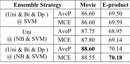
5.2.3 Different Ensemble Strategies
We also examine the performance of d
strategies. In Table 6, three ensemble strategies are compared, where “(Uni & Bi & Dp ) @ SVM” denotes ensemble of three kinds of fea-ture sets with the fixed SVM classifier, “Uni @ (NB & SVM)” denotes ensemble of two classi-fiers on fixed unigram features, and “(Uni & Bi & Dp ) @ (NB & SVM)” denotes ensemble of both classifiers and feature sets.
Ensemble Strategy Movie E-product
AveP 86.60 69.50 (Uni & Bi & Dp )
E
@ SVM MC 86.60 69.59
AveP 87.75 68.95 Uni
@ (NB & SVM) MCE 87.80 69.14
AveP 88.60 70.14
(Uni & Dp )
@ (NB & SVM) Bi &
MCE 88.55 70.18
Table 6: Accuracies Di Ens
Strategies.
f ensemble of either s or classifiers is ro
rams ovie
e-lin
t result (0.679) on joint features of un
for GWR of MI and
-se
(%) of fferent emble
Seen from Table 5 and 6, the performance o feature set
bustly better than any individual classifier, as well as the joint features on both datasets. With regard to ensemble of both feature sets and clas-sification algorithms, it is the most effective compared to the above two ensemble strategies.
This is in accordance with our motivation de-scribed in Section 3.1.
5.2.4 Comparison with Related Work
We take the performance of SVM on unig as the baseline for comparison. On the M dataset, Pang and Lee (2004) and Ng et al. (2006) reported the baseline accuracy of 0.871. But our baseline is 2 percentages lower (0.852). It is mainly due to that: 1) 0.871 was obtained by a 10-fold cross validation, and our result is get by 5-fold cross validation; 2) the result of the tool LibSVM is inferior of SVMlight by al-most 1-2 percentages, since the penalty parame-ter in LibSVM is fixed, while in SVMlight, the value is automatically adapted; 3) the baseline in Ng et al. (2006) is obtained with length nor-malization which play a role in performance.
Ng et al. reported the state of art best per-formance (0.905), which outperforms the bas
e (0.871) by 3.4%. Our best result of ensem-ble model (0.886) gets a comparaensem-ble improve-ment (3.40%) compared to our obtained base-line (0.852).
On the E-product dataset, Joshi and Rosé re-ported the bes
igrams and their proposed GWR features. This is in accordance with our result of Joint Features (0.6655 by SVM and 0.6764 by NB). The superiority of our ensemble result is quite significant (0.7014 by AvgP and 0.7018 by MCE).
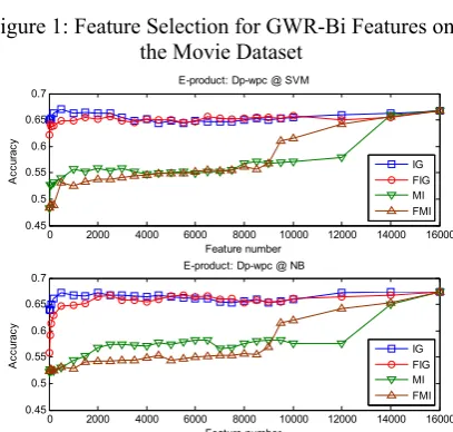
5.3 Results of Feature Selection
In this part, we examine FMI and FIG feature selection. The performance
IG are also presented for comparison. The re-sults on the Movie and E-product datasets are displayed in Figures 1 and 2 respectively. Due to space limit, we only report the results of GWR-Bi features for Movie and GWR-Dp fea-tures for E-product. In each of the figures, the results under NB and SVM are both presented.
At first, we observe the results of feature se-lection for GWR-Bi features on the Movie data
respectively, even better than the score with all features (0.8415).
0 10,000 20,000 30,000 40,000 50,000 60,000 70,000 80,000 90,000 150,000 0.6
Movie: Bi-wpc @ SVM
Feature number
0 10,000 20,000 30,000 40,000 50,000 60,000 70,000 80,000 90,000 150,000 0.6
Movie: Bi-wpc @ NB
Feature number
Figure 1: Feature Selection for GWR-Bi Features on the Movie Dataset
0 2000 4000 6000 8000 10000 12000 14000 16000 0.45
E-product: Dp-wpc @ SVM
Feature number
0 2000 4000 6000 8000 10000 12000 14000 16000 0.45
0.5 0.55 0.6 0.65
0.7 E-product: Dp-wpc @ NB
Feature number
A
ccu
ra
cy WR features for sentiment classification. We
have proposed a GWR feature extraction ap-proach and an ensemble model to efficiently integrate different types of features. Moreover, we have proposed two fast feature selection methods (FMI and FIG) for GWR features.
Individual GWR features outperform tr
IG FIG MI FMI
Figure 2: Feature Selection for GWR-Dp features on
We then ob finer granu-la
er-fo
size of E-pr
omparisons are made ac-co
he compu
ble model, when per-o
6
Conclusions and Future Work
adi-tio
proved to be a good solution for se-lecting GWR features. It is also worthy noting
stu
the E-product dataset
serve IG vs. FIG in a
rity. When the selected features are few (less than 5%), IG performs significantly better than FIG, while the latter gradually approaches the former when the feature number increases: as it comes to 10-15%, their performance is quite close. From then on, FIG is consistently compa-rable to IG, even sometimes slightly better.
With regard to MI and FMI, although the p rmance compared to IG and FIG is rather poor (the reason has been intensively studied by Yang and Pedersen, 1997). Our focus is the ability of FMI for approximating MI. From this point of view, FMI is by contrast effective, es-pecially with more than 1/3 features.
Compared to the Movie dataset, the
oduct dataset is much smaller, and the data are much sparser. Nevertheless, IG and FIG are
still effective. On one hand, top 1.25% (2000) features ranked by IG yield a result better than (or comparable to) that with all features. On the other hand, FIG is still competent to be a good approximation to IG.
All of the above c
rding to accuracies, and we now pay attention to computational efficiency. Taking the Movie dataset for example, IG needs to compute scores of information gain for all 152k features, while FIG only needs to comput k q5 5 scores, saving more than 70% of t tational load; on the E-product dataset, although the data are sparse, the rate of computation reduction is still significant (62.5%).
Note that in the ensem e 42
f rming FIG for individual GWR feature set, part of its inherent complexity is already taken care of by having already computed IG on Uni feature set, and we only need to compute the scores for 25 POS pairs. From this perspective, FIG is even more attractive in the ensemble model.
The focus of this paper is exploring the use of
nal WR features significantly, but they still can not totally substitute unigrams. The ensem-ble model is quite effective at integrating uni-grams and different types of WR feature, and the performance is significantly better than joint features.
FIG is
that FIG is a general feature selection method for bigram features, even outside the scope of sentiment classification and text classification.
Acknowledgment
We thank Yufeng Chen, Shoushan Li, Ping Jian and the anonymous reviewers for valuable com-ments and helpful suggestions. The research work has been partially funded by the Natural Science Foundation of China under Grant No. 60975053, 90820303 and 60736014, the Na-tional Key Technology R&D Program under Grant No. 2006BAH03B02, the Hi-Tech Re-search and Development Program (“863” Pro-gram) of China under Grant No. 2006AA010108-4, and also supported by the China-Singapore Institute of Digital Media (CSIDM) project under grant No. CSIDM-200804.
References
Kushal Dave, Steve Lawrence and David M. Pen-nock, 2003. Mining the Peanut Gallery: Opinion Extraction and Semantic Classification of Product Reviews. In Proceedings of the international World Wide Web Conference (WWW), pages 519-528.
Sašo Džeroski and Bernard Ženko, 2004. Is combin-ing classifiers with stackcombin-ing better than selectcombin-ing the best one? Machine Learning, 54 (3). pages 255-273.
Yoav Freund and Robert E. Schapire, 1999. Large margin classification using the perceptron algo-rithm. Machine Learning, 37 (3). pages 277-296.
Michael Gamon, 2004. Sentiment classification on customer feedback data: noisy data, large feature vectors, and the role of linguistic analysis. In Pro-ceedings of the International Conference on Com-putational Linguistics (COLING). pages 841-847.
Minqing Hu and Bing Liu, 2004. Mining and sum-marizing customer reviews. In Proceedings of the ACM SIGKDD Conference on Knowledge Dis-covery and Data Mining (KDD), pages 168-177.
Mahesh Joshi and Carolyn Penstein-Rosé, 2009. Generalizing dependency features for opinion mining. In Proceedings of the Joint Conference of the 47th Annual Meeting of the Association for Computational Linguistics (ACL), pages 313-316.
Biing-Hwang Juang and Shigeru Katagiri, 1992. Discriminative learning for minimum error classi-fication. IEEE Transactions on Signal Processing, 40 (12). pages 3043-3054.
J Kittler, 1998. Combining classifiers: A theoretical framework. Pattern Analysis and Applications, 1 (1). pages 18-27.
Shoushan Li, Rui Xia, Chengqing Zong and Chu-Ren Huang, 2009. A framework of feature selec-tion methods for text categorizaselec-tion. In Proceed-ings of the Joint Conference of the 47th Annual Meeting of the Association for Computational Linguistics (ACL), pages 692-700.
Andrew McCallum and Kamal Nigam, 1998. A com-parison of event models for naive bayes text clas-sification. In Proceedings of the AAAI workshop on learning for text categorization.
Vincent Ng, Sajib Dasgupta and S. M. Niaz Arifin, 2006. Examining the Role of Linguistic Knowl-edge Sources in the Automatic Identification and Classification of Reviews. In Proceedings of the COLING/ACL, pages 611-618.
Bo Pang and Lillian Lee, 2004. A Sentimental Edu-cation: Sentiment Analysis Using Subjectivity Summarization Based on Minimum Cuts. In Pro-ceedings of the Association for Computational Linguistics (ACL), pages 271-278.
Bo Pang and Lillian Lee, 2008. Opinion mining and sentiment analysis. Foundations and Trends in In-formation Retrieval, 2 (1-2). pages 1-135.
Bo Pang, Lillian Lee and Shivakumar Vaithyanathan, 2002. Thumbs up? Sentiment Classification using Machine Learning Techniques. In Proceedings of the Conference on Empirical Methods in Natural Language Processing (EMNLP), pages 79-86.