A Deep Convolutional Network for Multi-Type Signal Detection in Spectrogram

A Deep Convolutional Network for Multi-Type

Signal Detection in Spectrogram

Weihao Li 1,2,_{*, Keren Wang} 2 _{and Ling You} 2

1 _{PLA Strategic Support Force Information Engineering University, Zhengzhou 450001, China}

2 _{National Key Laboratory of Science and Technology on Blind Signal Processing, Chengdu 610041, China;} [email protected] (K.W.); [email protected] (L.Y.)

* Correspondence: [email protected]

Abstract: Wideband signal detection is an important problem in wireless communication. With the

rapid development of deep learning (DL) technology, some DL-based methods are applied to wireless technology, and the effect is obvious. In this paper, we propose a novel neural network for multi-type signal detection that can locate signals and recognize signal types in wideband spectrogram. Our network utilizes the key point estimation to locate the rough centerline of signal region and identify class. Then, several regressions are carried out to achieve properties, such as local offset and border offsets of bounding box, which is further synthesized for a more fine location. Experimental results demonstrate that our method performs more accurate than other DL-based object detection methods previously employed for the same detection task. Specifically, our method runs obviously faster than existing methods, and abandons the anchor generation, which makes it more favorable for real-time applications.

Keywords: deep learning; signal detection; wideband spectrogram; centerline

1. Introduction

Wireless communication plays an import role in military and civilian with its flexibility and long-distance transmission capability. The fast development of wireless communication and technology makes electromagnetic environment chaotic. Cognitive radio technology capable of learning and adapting to environment has attracted a lot of attention [1,2]. Signal detection (SD) mainly refers to detect the presence of multi-type signals or a specific signal in spectrum, hence being an important task in cognitive radio.

For traditional SD methods, energy detection has once been the most popular technique that can be classified as threshold-based algorithms [3–8] and non-threshold-based algorithms [9–13]. The method is to detect the energy of certain features to judge the presence of signals. Threshold-based algorithms set an experimental threshold to separate signal and noise, which has a relatively low computational requirements, but sensitive to noise and environmental changes. Non-threshold-based algorithms improve the universality of method, at cost of computational complexity. The effect of traditional methods is obvious, but some difficulties still limit the performance of algorithms. In practice, the prior information of received signals is usually unavailable. Especially in the wideband, carrier frequencies of signals are unknown, and bandwidth and duration vary with different signals. Most methods can only detect the presence of signal, needing subsequent algorithms to classify type, which is a complex process that needs expert knowledge. Moreover, the inference of noisy and irrelevant signals is unstable, which is a major problem faced by SD.

Recently, since the novel deep learning (DL) technology performs very well in computer vision, speech recognition, and natural language processing, it has also been introduced to wireless signal processing. By building deep neural network, DL method can learn high-dimensional features of input data. From this, it effectively improves recognition ability and reduces manual design. In addition, via enriching the characteristics of training data, the network is able to adapt to different environment and signal-to-noise ratio (SNR). [14,15] adopt convolutional neural network (CNN) + long short-term memory network (LSTM) and deep belief network (DBN) respectively to detect

signal in narrow band, with the input of raw data and spectral correlation function (SCF). Those methods only detect the presence of signals in a narrowband, without prediction of specific time-frequency parameters. [16] seeks out the narrowband fragments that contain signals from wideband spectrogram by energy detection, then utilizes CNN to perform recognition to obtain the wanted morse signal. It achieves signal detection and recognition in wideband spectrogram, but not a unified deep learning framework and the processing is multi-stage.

The time-frequency characteristic is commonly used for wireless signal processing. By calculating the spectrogram, time-frequency distribution and energy strength of signals can be clearly visualized, and many signal types are distinguishable in spectrogram, which also helps to signal recognition. In addition, some follow-up tasks of detected signal are usually based on the spectrogram, for example, the decoding of morse signal. In this paper, we detect the specific location of signals in wideband spectrogram, including start and end time and frequency, and identify the signals type. In fact, we convert SD task to an image object detection task, which can exploits the advantages of DL in computer vision to handle with. We construct a deep convolutional network that able to implement end-to-end training. Since the signal region in spectrogram is usually a horizontally-long rectangle, our network models signal by the centerline of its region, where signal type and a bounding box that completely surrounds the entire signal are regressed from the features at centerline. Compared to most object detection methods, our network abandons the candidate anchors generation and uses centerline instead of just a point to do predictions, which is more efficient and task-oriented (we will explain those in detail in section 2). Experimental results show our method has better detection accuracy, especially for the extremely long and closed spaced instances. Moreover, the simplicity of our network allows it to run at a very high speed.

To sum up, the main contribution of our work is: (1) We utilize the idea of DL-based object detection for multi-type SD in wideband spectrogram, capable of boxing location and recognizing signal type. (2) Different from directly applying commonly used object detectors, we targeting the characteristics of signal in spectrogram, propose a deep convolutional network that uses centerline to locate multi-type signal and abandons candidate anchors, which makes our method more accurate and faster.

2. Related Work

We want to accomplish multi-type SD in spectrogram by the idea of DL-based object detection. However, we think traditional detectors are not suitable for our task. Before us, the researchers in [17,18] have used the single shot multibox detector (SSD) which is a commonly used detector to perform SD, but the detection result is dissatisfactory, especially for the extremely long instance. In this section, we interpret the defects of traditional detectors for SD, and then raise our centerline-based method.

2.1. Defects of Traditional DL-Based Object Detectors

Most DL-based object detectors [19–24] achieve good performance when objects have regular shapes and aspect ratios. Nevertheless, the signal in spectrogram usually has extremely long shape, and time duration and frequency band vary dramatically with different signals, which makes it quite different from general objects. Those methods tend to get frustrated, and two main reasons are as considered: (1) Due to the limited receptive field of CNNs, some one-point based detectors [21,23,24] that use only one point or small area to predict box size cannot get complete bounding box; (2) The shapes of anchors of anchor-based methods [19–23] cannot fully encompass that of the signals, and anchors generation and regression are quiet time-consuming.

(a) (b)

Figure 1. Two typical defects of traditional DL-based detectors. (a) Limited receptive field of one point;

(b) Shape mismatch between anchors and ground truth boxes.

2.2. Signal as Centerline

In order to settle above problems, we propose to model signal as its centerline. Since signal region is usually a horizontally-long rectangle, we first find the centerlines to locate every signal, and utilize features in centerline to predict box size and signal type. The receptive field of centerline can easily cover entire signal, and we abandon anchor generation, turning to directly predict the offsets between centerline and up/down border lines, which avoids shape mismatch of anchors and saves a lot of time. The principle of our method is visualized in Figure 2.

Figure 2. Modeling signal as centerline. The box size and signal type are inferred from the features at

centerline.

3. Data Generation

The amount and richness of dataset is crucial for the training of deep neural networks, but the actually received wideband data we have is limited. Radio communication is a special case, whose signal transmission modality has a clear mathematical expression. So we simulate wideband signals by program, and introduce the process of data generating in this section, which indicates our simulation is quite meaningful.

We select 2FSK, 4FSK, PSK/QAM, morse, speech, and resident noise (RN) as the tested types of signal that are common in wideband. The above types of signals are intuitively distinguishable in the spectrogram except MPSK and MQAM, so we merge those two types to PSK/QAM. If we want to further identify MPSK and MQAM, some post-processing methods such as [17,25–27] can be introduced.

3.1. Expression of Multi-Type Signal

The transmitted digital modulation signal can be presented as:

( )

( ) j nt ( )

n b

n

s t 



where a is the transmitted symbols, _n n is the angular frequency,  is the carrier initial phase,

( )

g t is the shaping filter, and T is the symbol period. _b

For MFSK signal, it can be presented as:

0 2

1, , 0,1,..., 1

n n

a i i M

M

  

     . (2)

For MPSK signal, it can be presented as:

2 /

0

, 0,1,..., 1,

j i M

n n

For MQAM signal, it can be presented as:

0

, 2 1, 0,1,..., 1

4 4

n n n

n n

n

a I jQ

M M

I Q i i

       _{    }    

. ₍₄₎

For morse, it can be presented as:

0

0,1,

n n

a    . (5)

For RN, it is referring to the irrelevant signal with long duration, narrow bandwidth, and random energy changes. Here we presented it as a single frequency signal with a random amplitude change:

0

0.5 ~ 1.5, , ( ) 1

n n

a    g t  . (6)

For speech, we directly modulate real-world audio data to different frequencies by amplitude modulation.

3.2. Wideband Spectrogram Generation

In the actual communication environment, received signals of most systems are expressed as the equation:

0

( ) *

0

( ) j nLot ( ( )) ( ) ( )

Clk Add

r t e



This takes into account the effects of many factors in the real world on the signal. n t represents _Lo( ) the residual carrier random walk process, nClk( )t represents the time deviation, h t is the time-( ) varying channel function, and n_Add( )t is the additive noise.

To make the synthetic data valuable enough, we simulate comprehensively in a way identical to real situation. On the one hand, pulse shaping and bit rate that suitable for corresponding modulation mode are set up, and real voice or text is modulated as transmitted data. On the other, a robust channel model is employed including time varying multi-path fading, random frequency walk drifting, and additive gaussian white noise. We pass synthetic wideband signals through the channel model to get the final experimental data.

To obtain spectrograms of wideband signals, we utilize the short-time fourier transform (STFT), which is a common time-frequency analysis method. The calculation of STFT is:

( j ) ( ) ( ) j m

n m

S e 



2

( ) | ( j )|

n n

P  S e , (9)

Figure 3. Wideband spectrogram with multi-type signals.

4. Approach

Our proposed network is mainly composed of CNNs that perform well in the image recognition. The CNNs learn features via non-linear transformations implemented as a series of nested layers that introduce several kernels to perform convolution over the input. Generally, the kernels are usually multidimensional arrays that can be updated by some algorithms [28]. In this section, we first give an overview of our network, then elaborate the two core modules, and finally present the details of training and inference.

4.1. Overview

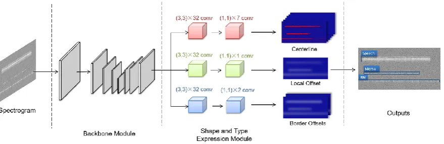
The overall architecture of our method is illustrated in Figure 4, which can be divided into two parts. First, we extract shared feature maps for subsequent tasks by backbone network. Our backbone network is ResNet18 with three up-convolution, where the feature maps of different stages are effectively merged. Then, we adopt a shape and type expression module (STEM), which utilizes the shared features to predict bounding box and signal type. The STEM construct a shape expression by learning geometry attributes including centerline, local offset and border offsets. The details of backbone module and STEM are presented as follow.

Figure 4. The proposed architecture.

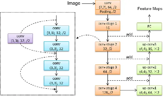
4.2. Backbone Module

problem during deep network training. We introduce three transposed convolution to up-sample the output of forward convolution, and each output of transposed convolution is added with that of corresponding convolutional stage. By merging the multi-scales feature maps, we can make full use of the input features at different level. The batch normalization and ReLU activation function are following the convolution layers, which are not marked in the figure.

Figure 5. Visualization of backbone module.

4.3. Shape and Expression Module

The STEM is a multi-channel convolutional network and can be divided to three branches. In each branch, we utilize 3 3 and 1 1 convolution layers with different channels to regress the signal property maps including centerline, local offset and border offsets.

Centerline is a 7 (6 signal types + 1 background) channels map that represents the pixel-wise

probability of the centerline of different classes. For the produce of ground truth centerline maps, we compute a low-resolution equivalent ~ p

R

p for each centerline point p of class c , then splat all ~

p onto a heatmap _[0,1]W HR RC

Y   using a gaussian kernel

~

~ 2 2

2

( ) ( )

2

exp( x y )

p

xyc

x p y p

Y



  

  , where [ , ]W H is the width and height of input image, R is the down-sampling scale, C is the number of

signal types,  is an object size-adaptive standard deviation. The training objective of centerline is pixel-wise focal loss:

^ ^

^ ^

(1 ) log( ), 1 1

(1 ) ( ) log(1 ),

xyc xyc _xyc

cl xyc

xyc xyc

xyc

Y Y if Y

L N

Y Y Y otherwise

            



where  and  are hyper parameters of the focal loss, and N is the number of centerline points in a spectrogram. Here we chose 2 and 4 in our all experiments.

Local offset is a 1 channel map that has valid values within the centerline. To recover the

discretization error caused by the down-sampling of backbone network, we additionally predict a vertical local offset _{O R}^  W HR R1_{. It will be added to the ordinate of centerline when mapping the}

shrunken image to original size. The training objective of local offset is the L1 loss at centerline points:

~

^ ~

1

| p ( y )|

off y

p

p

L O p

N R





Border offsets is a 2 channels map that has valid values within the centerline. The value of two

channels y( )up~ ,

~

( )p d

y correspond to the offsets between centerline and up/down border lines.

~ ~

~

^ _{( )p ( )p}

p u d

S y y is the predicted height of box at p . The truth width at p is ~ Sp, so just like the local

~

^

1

| p |

border p

p

L S S

N





Bounding box and signal type generation: We have got the predicted centerline, local offset,

and border offsets at each pixel, and need to determine the final bounding box and signal type. We set a threshold on the heat map to obtain all of the positive centerline connected domain. Each connected domain corresponds to a signal, and the pixel class that appears most frequently in a domain is the predicted type of signal. The horizontal minimum x^min and maximum

^ max x of connected domain is the time start and stop. We chose the row with the largest cumulative probability of predicted class in each connected domain as the final centerline. The average of local offset and border offsets at the centerline are the final predicted values. So we can obtain coordinates of the lower left and upper right corner of bounding box as follow:

^ ^

^ ^ ^ ^ ^ ^

min max

( , _d, , _u)

R x y O y x  y O y  . (13)

As we can see, all bounding boxes are produced directly from the centerline estimation without the need of de-redundant processes such as intersect over union (IOU)-based non-maxima suppression (NMS). The architecture of our model is simple and elegant, compared to most traditional two-stage or one-stage object detection models.

4.4. Training and Inference Details

We train the proposed network end-to-end with the following loss function:

1 cl 2 off 3 border

LL L L . (14)

Total loss is a weighted sum of the three property losses. The weights 1, 2, 3 that trade off

among three losses are set to 1.0, 0.5, 0.5 in our experiments.

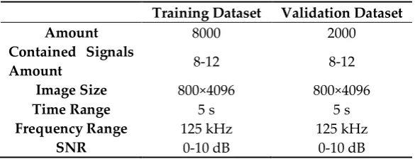
To make training more efficient and effective, we randomly crop and scale the input image to different sizes, and add gaussian noise. The details of training and validation dataset are presented in Table 1. The Adam optimizer with a learning rate of 2e-4 is used to optimize the overall objective. We train with a batch size of 50 for 150 epochs and all experiments are performed on a Tesla P40 GPU.

Table 1. Training and validation dataset details.

Training Dataset Validation Dataset

Amount 8000 2000

Contained Signals

Amount 8-12 8-12

Image Size 800×4096 800×4096

Time Range 5 s 5 s

Frequency Range 125 kHz 125 kHz

SNR 0-10 dB 0-10 dB

5. Experiments

5.1. Comparative Experiment

Researchers in [17] exploit SSD and Fast-RCNN [19] to detect signals in spectrogram, which suggests that Fast-RCNN has a good precision (we can expect that the Faster-RCNN could do better than Fast-RCNN), while SSD is deft at speed. Here we compare different methods in precision and speed. Precision metric is mean Average Precision (mAP) [29], the mean of different classes’ AP. AP comprehensively represents the predicted precision and recall of one object class at a given IOU threshold. Speed metric is frame per second (FPS), representing the number of images that model can process per second.

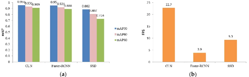
The backbones of experimental SSD and Faster-RCNN are both VGG-16 [30]. In order to ensure the fairness of comparison, for SSD and Faster-RCNN, we use the same training methods, data augmentation and so on as our network. Those three models are trained to convergence. Figure 6 shows the quantitative comparison of detection accuracy and speed. CLN has the best accuracy in different IOU threshold, while Faster-RCNN is the second, and SSD is a little bit worse. Results demonstrate our centerline-based approach is more suitable for signal than the one-point based methods as the other two. In terms of processing speed, CLN shows an obvious advantage, even for the fast SSD model. Because our method discards the process of anchors generation and NMS, detection speed is greatly improves.

(a) (b)

Figure 6. Quantitative comparison results of different methods. (a) Comparison of mAP; (b)

Comparison of FPS. mAP50, mAP60, mAP80 represent the mAP at IOU threshold 0.5, 0.6, 0.8. FPS is tested on a Tesla P40 GPU.

To further visualize and analyze the performance, in Figure 7 we randomly plot some detection results of three methods. Figure 7(a) is the result of CLN that able to traces out precise bounding box containing the whole signal, and successfully identifies types with a high confidence score. Benefit from twice boundary regression, Faster-RCNN also has a nice detection and recognition performance in Figure 7(b), but it occasionally confuses two signals that are very close to each other (the speeches in the bottom spectrogram). In Figure 7(c), although SSD has found the presence of signals, but fails to draw up complete bounding box, especially for the extremely long instances.

(a) (b) (c)

Figure 7. Detection results of three methods. (a) Results of CLN; (b) Results of Faster-RCNN; (c)

Results of SSD.

5.2. Additional Experiments

The input data of our network is spectrogram, so to evaluate the robustness, we carry out sensitive tests on some factors able to influence the representation of signals in the spectrogram.

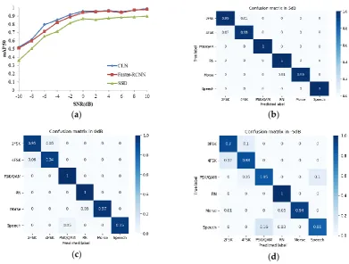
Different SNR: Figure 8(a) shows the detection mAP50 versus -10-10dB SNR of three methods.

(a) (b)

(c) _(d)

Figure 8. Detection performance in different SNR. (a) Detection mAP50 vs. SNR of three models; (b)

- (d): Confusion matrixes of CLN in 5dB, 0dB, -5dB respectively.

Different frequency resolution: The frequency resolution is an important and necessary

argument for spectrogram expression. To test the robustness to frequency resolution, we vary it from 20 Hz to 40 Hz to evaluate detection performance. In Figure 9, the mAP50 curves of different methods are drawn in different colors. Generally, all models perform best in 30 Hz, since our training frequency resolution is about 30.5 Hz. When reducing or increasing frequency resolution, the detection effect does not fluctuate obviously. So the change of resolution in a certain range has limited impact on detection effect. This may be because that in those cases, signals of different types can still be intuitively distinguished in spectrogram.

Figure 9. Detection performance vs. frequency resolution.

Height of ground truth box: During our dataset generation in 3.2, we annotate with boxes whose

Faster-RCNN and SSD to [1/2, 1/10, 1/15, 1/20]. The detection results are presented in Figure 10, and we can see that our method is still able to regress the boxes closed to ground truth, but the performance of SSD and Faster-RCNN is greatly reduced, especially the missing and redundant predictions.

For our method, it focuses on the centerline of signal that does not change with the height of annotated box, only needing to predict different border offsets. For SSD and Faster-RCNN, since the size and aspect ratio of boxes differs quite a lot for different signals, it is difficult to design a group of common anchors. Some ground truth boxes may miss match with candidate anchors during input encoding, in addition, those signals with small bandwidth or long duration may get repeated but no overlapping predictions, which cannot be get rid of by IOU-based measures like NMS. So if you want to use the anchor-based methods to detect signals in spectrogram, you had better adjust the anchors well and annotate with higher ground truth boxes.

(a) (b) (c) (d)

Figure 10. Detection results with the annotated box height close to signal bandwidth. (a) Ground truth

boxes; (b) Results of CLN; (c) Results of Faster-RCNN; (d) Results of SSD.

6. Conclusions

In this paper, we present a deep convolutional network for multi-type SD in the wideband spectrogram. We analyze the defects of directly applying DL-based object detectors to SD, and propose a centerline-based method. The method targeting the characteristics of signal, first finds the centerlines of signal region, then regresses to complete box and class identification. In experiments, we have carried out comparison with other object detection methods in accuracy and speed, and sensitive tests in different SNR, frequency resolution and annotated box height. The results indicate that our method has high detection mAP with an obvious speed advantage. It also has a good robustness under the change of above influence factors. In addition, the no need of anchor design or post-processing like NMS makes our method simple and efficient to deploy.

In the future, we plan to extend our dataset, and explore more comprehensive features for signal detection and recognition.

References

1. Khan, A.A.; Rehmani, M.H.; Reisslein, M. Cognitive Radio for Smart Grids: Survey of Architectures,

Spectrum Sensing Mechanisms, and Networking Protocols. IEEE Commun. Surv. Tutor. 2015, 18, 1-1. Doi:

2. Joshi, G.P.; Nam, S.Y.; Kim, S.W. Cognitive Radio Wireless Sensor Networks: Applications, Challenges and

Research Trends. Sensors 2013, 13, 11196-11228. Doi: 10.3390/s130911196

3. Salt, J.E.; Nguyen, H.H. Performance prediction for energy detection of unknown signals. IEEE Trans. Veh.

Technol. 2008, 57, 3900-3904. Doi: 10.1109/TVT.2008.921617

4. Urkowitz, H. Energy detection of unknown deterministic signals. Proc. IEEE 1967, 55, 523-531. Doi:

10.1109/PROC.1967.5573

5. Lehtomaki, J.J.; Vartiainen, J.; Juntti, M.; Saarnisaari, H. Analysis of the LAD Methods. IEEE Signal Process.

Lett. 2008, 15, 237-240. Doi: 10.1109/LSP.2008.916729

6. Lehtomaki, J.J.; Vartiainen, J.; Juntti, M.; Saarnisaari, H. CFAR Outlier Detection With Forward Methods.

IEEE Trans. Signal Process. 2007, 55, 4702-4706. Doi: 10.1109/tsp.2007.896239

7. Tadaion, A.A.; Derakhtian, M.; Gazor, S.; Nayebi, M.M.; Aref, M.R. Signal Activity Detection of Phase-Shift

Keying Signals. IEEE Trans. Commun. 2006, 54, p.1439-1445. Doi: 10.1109/tcomm.2006.876884

8. Salembier, P.; Liesegang, S.; López-Martínez, C. Ship detection in SAR images based on maxtree

representation and graph signal processing. IEEE Trans. Geosci. Remote Sensing 2018, 57, 2709-2724. Doi:

10.1109/TGRS.2018.2876603

9. Bao, D.; De Vito, L.; Rapuano, S. A Histogram-Based Segmentation Method for Wideband Spectrum

Sensing in Cognitive Radios. IEEE Trans. Instrum. Meas. 2013, 62, 1900-1908. Doi: 10.1109/TIM.2013.2251821

10. Bao, D.; De Vito, L.; Rapuano, S. Spectrum segmentation for wideband sensing of radio signals. In

Proceedings of 2011 IEEE International Workshop on Measurements and Networking Proceedings (M&N),

Anacapri, Italy, 2011; pp. 47-52. Doi: 10.1109/IWMN.2011.6088506

11. Koley, S.; Mirza, V.; Islam, S.; Mitra, D. Gradient-based real-time spectrum sensing at low SNR. IEEE

Commun. Lett. 2014, 19, 391-394. Doi: 10.1109/LCOMM.2014.2387168

12. Men, S.; Chargé, P.; Wang, Y.; Li, J. Wideband signal detection for cognitive radio applications with limited

resources. EURASIP J. Adv. Signal Process. 2019, 2019, 2. Doi: 10.1186/s13634-018-0600-6

13. Dibal, P.; Onwuka, E.; Agajo, J.; Alenoghena, C. Wideband spectrum sensing in cognitive radio using

discrete wavelet packet transform and principal component analysis. Phys. Commun. 2020, 38, 100918. Doi:

10.1016/j.phycom.2019.100918

14. Ke, D.; Huang, Z.; Wang, X.; Li, X. Blind Detection Techniques for Non-Cooperative Communication

Signals Based on Deep Learning. IEEE Access 2019, 7, 89218-89225. Doi: 10.1109/access.2019.2926296

15. Mendis, G.J.; Wei, J.; Madanayake, A. Deep Learning based Radio-Signal Identification with Hardware

Design. IEEE Trans. Aerosp. Electron. Syst. 2019, 55, 1-1. Doi: 10.1109/TAES.2019.2891155

16. Yuan, Y.; Sun, Z.; Wei, Z.; Jia, K. DeepMorse: A Deep Convolutional Learning Method for Blind Morse

Signal Detection in Wideband Wireless Spectrum. IEEE Access 2019, 7, 80577-80587. Doi:

10.1109/ACCESS.2019.2923084

17. Zha, X.; Peng, H.; Qin, X.; Li, G.; Yang, S. A Deep Learning Framework for Signal Detection and Modulation

Classification. Sensors 2019, 19, 4042. Doi: 10.3390/s19184042

18. Yang S., Jin S., Peng H., Hou X., Fu J., Ultra－Short wave specific signal detection and recognition based on

spectrogram and deep convolution neural network, J. Information Engineering University 2019, 20.

19. Girshick, R. Fast r-cnn. In Proceedings of the IEEE international conference on computer vision, Santiago,

Chile, 7–13 December 2015; pp. 1440–1448. Doi: 10.1109/ICCV.2015.169

20. Ren, S.; He, K.; Girshick, R.; Sun, J. Faster r-cnn: Towards real-time object detection with region proposal

21. Liu W., Anguelov D., Erhan D., Szegedy C., Reed S., Fu C., Berg A., SSD: Single shot multibox detector. In

Proceedings of the 14th European Conference ECCV 2016, Amsterdam, The Netherlands, 11–14 October 2016;

pp. 21–37. Doi: 10.1007/978-3-319-46448-0_2

22. Redmon J., Farhadi A., YOLOV3: An incremental improvement. arXiv 2016, arXiv:1612.08242.

23. Lin, T.-Y.; Goyal, P.; Girshick, R.; He, K.; Dollár, P. Focal loss for dense object detection. In Proceedings of

the IEEE international conference on computer vision, 2017; pp. 2980-2988. Doi:

10.1109/TPAMI.2018.2858826

24. Zhou, X.; Wang, D.; Krähenbühl, P. Objects as points. arXiv 2019, arXiv:1904.07850 2019.

25. Kim, B.; Kim, J.; Chae, H.; Yoon, D.; Choi, J.W. Deep neural network-based automatic modulation

classification technique. In Proceedings of 2016 International Conference on Information and

Communication Technology Convergence (ICTC), Jeju, South Korea, 2016; pp. 579-582. Doi:

10.1109/ictc.2016.7763537

26. Ali, A.; Yangyu, F. Unsupervised feature learning and automatic modulation classification using deep

learning model. Phys. Commun. 2017, 25, 75-84. Doi: 10.1016/j.phycom.2017.09.004

27. O’Shea, T.J.; Corgan, J.; Clancy, T.C. Convolutional radio modulation recognition networks. In Proceedings

of International conference on engineering applications of neural networks, Cham, Switzerland, 2016; pp.

213-226. Doi: 10.1007/978-3-319-44188-7_16

28. LeCun, Y.; Bottou, L.; Bengio, Y.; Haffner, P. Gradient-based learning applied to document recognition.

Proc. IEEE 1998, 86, 2278-2324. Doi: 10.1109/5.726791

29. Everingham, M.; Eslami, S.A.; Van Gool, L.; Williams, C.K.; Winn, J.; Zisserman, A. The pascal visual object

classes challenge: A retrospective. Int. J. Comput. Vis. 2015, 111, 98-136. Doi: 10.1007/s11263-014-0733-5

30. Simonyan, K.; Zisserman, A. Very deep convolutional networks for large-scale image recognition. arXiv