Article
Reach On Waste Classification and Identification by
Transfer Learning and Lightweight Neural Network
Xiujie Xu 1, Xuehai Qi 1,*,Xingjian Diao21 School of Management Engineering, Shandong Jianzhu University, Jinan 250101, China;[email protected]
2 University of Pittsburgh, Computer Science Major,4200 Fifth Ave, Pittsburgh, PA 15260, United States,
* Correspondence: [email protected]; Tel.: +86-178-6512-5895
Abstract: Using machine learning or deep learning to solve the problem of garbage recognition and classification is an important application in computer vision, but due to the incomplete establishment of garbage datasets and the poor performance of complex network models on smart terminal devices, the existing garbage classification models The effect is not good.This paper
presents a waste classification and identification method base on transfer learning and lightweight
neural network. By migrating the lightweight neural network MobileNetV2 and rebuild it, The reconstructed network is used for feature extraction, and the extracted features are introduced into the SVM to realize the identification of 6 types of garbage. The model was trained and verified by using 2527 pieces of garbage labeled data in the TrashNet dataset, which ultimately resulted in a classification accuracy of 98.4% of the method, which proves that the method can effectively improve the classification accuracy and time and overcome the problem of weak data and less labeling. The over-fitting phenomenon encountered by small data sets in deep learning makes the model robust.
Keywords: Waste classification; Transfer learning; Deep learning; Recognition classification
1. Introduction
With the development of China's economy, and the acceleration of urbanization, the threat of solid waste to the ecological environment is increasing. In July 2019, the British company Verisk Maplecroft pointed out in a research report of "Waste generation and recycling indices 2019". Every year, the total amount of solid waste generated in cities worldwide exceeds 2.1 billion tons, of which only 16% can be recycled, and nearly half of them are abandoned and cannot be recycled. Although China's per capita production of solid waste is less than that of the United States, Canada, and Western European countries, the total amount of solid waste is much more significant than that of India and the United States, which ranks second and third. The total amount accounts for 15% of the global urban garbage.
In 2019, Shanghai issued the regulations of the Shanghai Municipality on the management of domestic garbage and began to implement the mandatory classification of garbage. Subsequently, Beijing, Taiyuan and other eight cities in China successively promulgated the regulations on the management of domestic waste, and incorporated waste classification into the legal framework.
Garbage classification is the most effective way to deal with pollution. By carefully classifying domestic waste and choosing economical and reasonable treatment methods based on the nature of the classified waste, not only can it reduce the investment and operating costs of waste treatment, but it can also reduce the environmental pollution and waste of land resources caused by waste treatment. At present, artificial waste classification is facing problems such as low efficiency, high cost, and difficulty in the promotion. The use of artificial intelligence terminal equipment to classify garbage has become a research hotspot and the development direction of the garbage industry.
In 2016, J. Donovan's team designed an automatic sorting bin based on the Raspberry Pi. This project is built using Google's Tensorflow framework, which can distinguish two categories of garbage[1]. In 2016, G. Mittal et al. Developed a mobile application that roughly divides a pile of junk in images. The data set used in this project was obtained through the Bing image search. By using a pre-trained AlexNet 1 model, the average accuracy was accurate. The rate was 87.69%[2]. In 2016, Thung G and others established Trashnet, a public data set that includes glass, paper, metal, plastic, cardboard, and other trash. On this data set, SVM is used to extract the features of the image, and the scratch-CNN network is used to classify the garbage. The test accuracy is 75%[3]. In 2018, Cenk et al. Achieved 95% test accuracy in the Trashnet dataset by applying models and data augmentation[4].
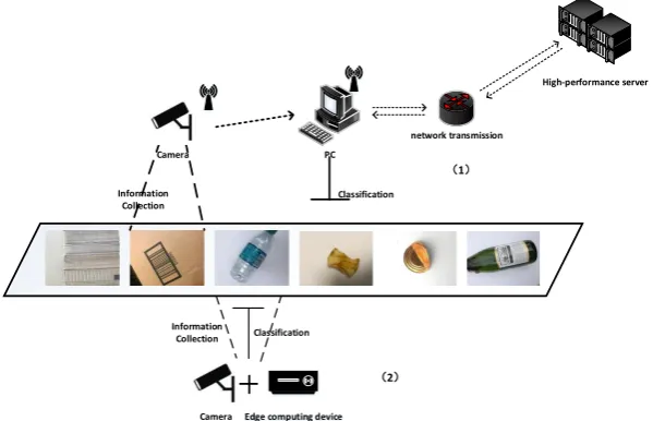
At present, there are two main working principles of artificial intelligence-based garbage recognition and classification terminal devices. One is to collect information based on information collection equipment such as cameras and sensors and rely on high-speed networks and high-performance servers to process data. The other is to deploy the model directly. On a terminal device equipped with an edge computing chip, the device handles the analysis by itself. The advantage of the first method is that the terminal equipment has low cost and high recognition accuracy, but the disadvantage is that it relies heavily on the network. Without the network, the device will not work correctly. The advantage of the second method is that it does not require a network and can be flexibly deployed. However, the disadvantage is that terminal equipment equipped with edge computing chips has a high cost and limited computing power, and has high requirements on the model itself. Figure 1 shows the two working principles.
PC
High-performance server
network transmission Camera
Classification Information
Collection
Edge computing device Camera
Information
Collection Classification
(1)
(2)
Figure 1. Two types of waste sorting equipment work
For the second type of garbage recognition and classification equipment, it is a development and research direction to improve the recognition accuracy and speed of the model and reduce the calculation cost.
In order to solve the problems such as low data, weak computing, and universalization of models in the current garbage classification and garbage identification and classification equipment, this research conducted a series of experimental tests using traditional machine learning and deep learning to summarize their advantages and disadvantages Finally, a waste classification and identification method based on transfer learning and lightweight neural network is proposed. By migrating the MobileNetV2 model and transforming it, the new model achieves better accuracy with fewer data and weak calculations. Compared with traditional machine learning and deep learning, the method proposed in this study has significant advantages in terms of recognition accuracy and training time.
2. Materials and Methods
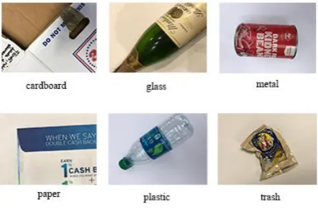
The data set used in this research is from Trashnet, a data set collected by Thung G et al. [5]Trashnet mainly includes glass, paper, cardboard, plastic, metal and daily garbage pictures in a total of 2527 six categories, including 501 glass, 594 paper, 403 cardboard, 482 plastic, 410 metal, 137 daily trash. An example of each type of garbage in the data set is shown in Figure 2.
Figure 2. TrashNet DataSet
2.2. Related theories
2.2.1. Machine learning
Since the 1980s, machine learning has indeed become an independent subject area. Since then, various machine learning algorithms have been proposed in large numbers and developed rapidly. In the early 1990s, Breiman, Quinlan, and others successfully proposed typical algorithms for decision trees such as CART[6], ID3[7], and C4.5[8]. Decision tree classifies data through a series of rules, which is a method to get what value based on what conditions. The decision tree algorithm is explainable and straightforward, which makes the decision tree algorithm still used in some problems.
In 2001, Breiman proposed a random forest algorithm which is the development of Bagging [9]. The random forest based on the decision tree-based learner to build Bagging integration, and it further introduces random attribute selection during the training of decision trees.
In 1995, Cortes and Vapnik proposed the support vector machine SVM[10]. The proposal of SVM represents the victory of Kernel technology. SVM uses kernel technology to map input vectors into high-dimensional space and divides the samples by dividing the hyperplane, making the original linearly inseparable problem linearly separable[11].
In 1901, Karl Pearson invented the principal component analysis (PCA)[12]. PCA is a commonly used data analysis method. PCA can be used to extract the main feature components of the data, which is often used to divide and reduce the dimensions of high-dimensional data[14]. The Kernel PCA algorithm appeared in 1998. The emergence of Kernel PCA as a non-linear dimensionality reduction algorithm is another victory for Kernel technology. The combination of Kernel PCA and PCA transforms PCA into a non-linear dimensionality reduction algorithm to handle higher-order correlations. Sexual data has excellent results.
2.2.2. Deep learning
point in deep learning. After 2012, deep neural networks made a comeback, and they began to be widely used in image and speech perception issues and achieved real breakthroughs. The development of deep learning is not accidental. He has a universal approximation theorem as a guarantee that it can fit any continuous function on a closed interval. In addition, he can manually control the size of the neural network to fit very complex functions. This is the original What machine learning algorithms do not have.
In 1989, LeCun designed the first genuinely convolutional neural network (CNN)[16], and first applied it to handwriting recognition. The main structure of a convolutional neural network consists of an input layer, a convolutional layer, a pooling layer, a fully connected layer, and an output layer. In ordinary neural networks, fully connected layers flatten multidimensional data. However, because the image is a 3-dimensional structure, flattening the image may ignore important information during processing or learning. The convolution layer can keep the shape unchanged. When processing image data, the convolutional layer receives data in the form of 3D data and and outputs it to the next layer in the same form. Convolutional layers allow models to learn data with shapes such as images correctly. Pooling can reduce spatial operations in high and long directions. The pooling layer can enlarge the features of the data transmitted from the convolution layer and reduce the parameters at the same time. There are no parameters to learn in the pooling layer. Figure 3 shows the structure of a convolutional neural network.
Figure 3. Convolutional neural network
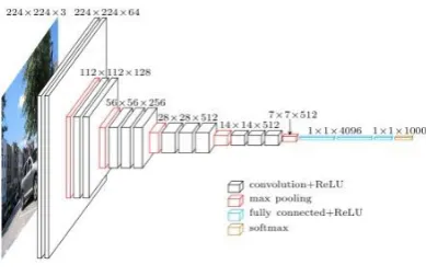
In 2014, researchers from the University of Oxford's and Google advanced a new deep convolutional neural network VGGNet[17] and won the second place and the first place in the ILSVRC2014 competition. The success of VGGNet proves that using the small convolution kernel instead of the large convolution kernel can produce better results. Because the multiple non-linear layers can improve the depth of the network to ensure that more patterns are learned, and at a lower cost, and it is concluded that the performance of the model can be effectively improved by increasing the depth of the network. Figure 4 shows the structure of the VGG network.
Figure 4. Visual Geometry Group
2.2.3. Transfer learning
deep learning has apparent advantages in processing massive data, big data, large equipment, and immense computing power are costly and are not suitable for the research and development of small and medium-sized enterprises. Big data, ample storage, and astronomical calculations make the accuracy of machine learning models better and better, but the generalization ability of models has not been significantly improved. A model trained with a lot of human and financial resources can often only solve specific problems, and often needs to restart training for different problems. On the one hand, this method is non-artificial and not artificial. On the other hand, this method is costly.
With the emergence of problems such as less annotation, weak computing, and generalization of models, the idea of transfer learning has been proposed. Transfer learning focuses on applying what has been learned to new problems. Its core is to find the similarity between the new problem and the original problem, to transfer knowledge.
With the popularity of deep learning, convolutional neural network models in the field of computer vision have emerged endlessly. The effect of deep learning network models in image processing is getting better and better, but at the same time the size of neural networks is getting larger and larger, the structure is getting more and more complex, and the hardware resources required for training and deployment are getting more and more. Due to the limitations of hardware resources and computing power of mobile devices, it is challenging to run deep learning network models to a certain extent. In the field of deep learning, efforts are also being made to promote the miniaturization of neural networks. From 2016 to the present, the industry has proposed lightweight network models such as SqueezeNet, ShuffleNet, NasNet, MnasNet, and MobileNet. These models make it possible for mobile terminals and embedded devices to run neural network models. MobileNet[19] is more representative in lightweight neural networks, which has a smaller network size, less computation, and higher accuracy.
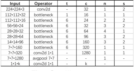
In March 2019, Google proposed MobileNetV2 network architecture[20]. MobileNetV2 is a lightweight network architecture based on MobileNetV1. It mainly introduces a linear bottleneck structure and reverses residual structure. There are a total of 17 Bottleneck layers in the MobileNetV2 network model (each Bottleneck contains two pointwise convolutional layers and a depth convolutional layer), a standard convolutional layer (Conv), and two pointwise convolutional layers (PW Conv) There are a total of 54 trainable parameter layers. MobileNetV2 uses Linear Bottleneck and Inverted Residuals structures to optimize the network, making the network deeper, but the model is smaller and faster. Figure 5 shows MobileNetV2.
Input Operator t c n s
224*224*3 conv2d - 32 1 2 112*112*32 bottleneck 1 16 1 1 112*112*16 bottleneck 6 24 2 2 56*56*24 bottleneck 6 32 3 2 28*28*32 bottleneck 6 64 4 1 28*28*64 bottleneck 6 96 3 2 14*14*96 bottleneck 6 160 3 2 7*7*160 bottleneck 6 320 1 1 7*7*320 conv2d 1*1 - 1280 1 1 7*7*1280 avgpool 7*7 - - 1
-1*1*k conv2d 1*1 - k
-Figure 5. MobileNetV2
2.3. Experimental environment
In the model verification and evaluation phase, this study uses a cross-validation method[22] to evaluate the performance of the model. Using cross-validation can effectively improve the generalization ability of the model and overcome the overfitting. Using ten-fold cross-validation, divide all data sets into ten copies, take one copy each time for testing and take nine copies for training, and finally obtain the mean.
The experimental environment of the machine learning part of this research is Windows 10 system, the processor is Intel (R) CoreTMi7-6700hq [email protected], and the running memory is 16GB. The code for this experiment was written on the jupyter notebook platform, based on the sklearn library, and implemented in Python 3.7.
The experimental environment of this study in the deep learning and transfer learning part is Ubuntu 18.04.3 LTS system. The processor is Intel (R) Xeon (R) CPU @ 2.30GHz, the operating memory is 25GB, and the graphics card is Tesla K80. The code for this experiment was written on the jupyter notebook platform, based on Tensorflow2, and implemented in Python 3.7.
3. Experiments and Results
Before verifying the method proposed in this study, this experiment first uses standard machine learning algorithms and deep learning models to train and test on the TrashNet dataset. The two methods are compared in terms of classification accuracy and training time, and their limitations and shortcomings are summarized.
3.1. Performance of the Machine learning on TrashNet Dataset
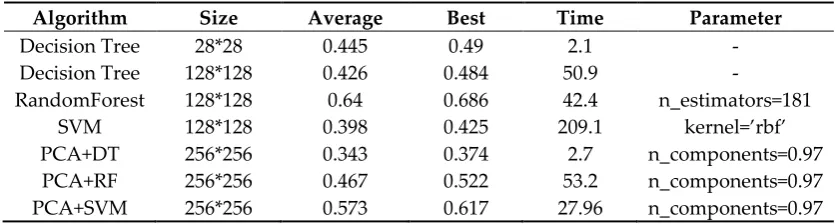
In the machine learning part, traditional machine learning algorithms such as decision trees, random forests, SVMs, and PCA are used to train and verify the data set. When using machine learning algorithms to process image data, most of them flatten 2D pictures to 1D and introduce 1D data into machine learning algorithms for training and classification. The size of the pictures in the TrashNet dataset is 384 * 512. When using a decision tree algorithm to model the dataset, it was found that proper reshaping of pictures can raise the accuracy and speed of classification. When the image size is reshaped to 28 * 28, the training time is 2.1 seconds, and the optimal score is 0.49. However, the 28 * 28 size picture cannot be recognized by human eyes. Figure 6 is the reshaped picture (28 * 28).
Figure 6. Photo reshape(28*28)
However, decision trees and random forest algorithms have fallen. The test results of the machine
learning algorithm are shown in Table 1..
Table 1. Result of Machine learning
Algorithm Size Average Best Time Parameter
Decision Tree 28*28 0.445 0.49 2.1 -
Decision Tree 128*128 0.426 0.484 50.9 -
RandomForest 128*128 0.64 0.686 42.4 n_estimators=181
SVM 128*128 0.398 0.425 209.1 kernel=’rbf’
PCA+DT 256*256 0.343 0.374 2.7 n_components=0.97
PCA+RF 256*256 0.467 0.522 53.2 n_components=0.97
PCA+SVM 256*256 0.573 0.617 27.96 n_components=0.97
3.2. Performance of the Deep learning on TrashNet Dataset
In the deep learning part, deep learning models such as a three-layer neural network, CNN network, and VGG16 are used to train and verify the data set. The size of the original picture of the dataset is 384 * 512. When testing with a deep learning model, the size of the input layer of the model is uniformly set to (384 * 512 * 3), the output layer is set to 6 types, and the activation function uses softmax. When using a three-layer neural network structure for training, since the hidden layer is still processing the flattened data, the classification effect is not apparent, and overfitting occurs. When using the CNN model for training, the model was trained 20 times in 316.5 seconds, and the optimal score was 0.6087, but in the process of long-term model training, the model was overfitted. The results of the CNN test, on the one hand, prove that the convolutional neural network is suitable for image classification problems, but using a small data set to train the neural network is very prone to overfitting. When using the deeper neural network VGG16, the model appeared overfitting earlier. It can be seen that complex models are not necessarily suitable for small data sets. The test results of the deep learning model are shown in Table 2.
Table 2. Result of Deep learning
Model Size Best time Epochs
Three-Layered Neual Networks 384*512 0.2609 51.1 20
CNN 384*512 0.6087 316.5 20
VGG16 384*512 0.2016 1342.4 20
3.3. Performance of the Transfer learning on TrashNet Dataset
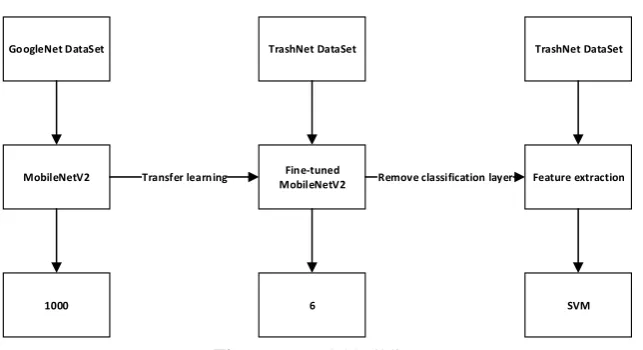
3.3.1. Model building
GoogleNet DataSet
MobileNetV2
1000
Transfer learning MobileNetV2Fine-tuned
6
Remove classification layer Feature extraction TrashNet DataSet
SVM TrashNet DataSet
Figure 6. Model building
3.3.2. Model testing
In the transfer learning test section, this study migrated two representative models, VGG16 and MobileNetV2, to train and test them, respectively. The number of parameters of the migrated VGG16 model is 14,717,766. By comparing the parameters of the multi-network deep VGG16 network, the classification accuracy and training score are lower than the light neural network MobileNetV2. SVM was fine-tuned at the end of the experiment. The best classification effect was 0.987 when the kernel function was selected as RBF, and the gamma was set to 0.15998587196060574. Table 3 compares the classification accuracy using transfer learning.
Table 3. Result of Transfer learning
Model Size Best time Epochs
VGG16+softmax 384*512 0.707 537.4 20
MobileNetV2+softmax 384*512 0.8814 50.5 10
MobileNetV2+SVM 384*512 0.987 50.5 10
4. Discussion
In order to verify the feasibility of the research method, the proposed method is compared with the traditional machine learning algorithm and deep learning model. In the traditional machine learning part, the recognition rates of decision trees and random forest algorithms are 0.49 and 0.68, respectively, which proves that decision trees and random forest algorithms are easy-to-use and straightforward algorithms for dealing with everyday problems, but the accuracy of the algorithm has limitations. SVM encountered a computational bottleneck because the data dimension was too high when processing the data set, and the effect was not apparent after using PCA to reduce the dimension. In the deep learning part, the performance of the three-layer neural network is weak. It can be seen that flattening the data when dealing with image problems does cause the loss of some picture information. When using models such as CNN and VGGNet, I encountered overfitting problems, which is indeed a common problem in deep learning when training with small samples. Finally, the recognition rate of the garbage recognition classification method based on the transfer learning and lightweight neural network proposed in this study is 98.4%. It is proved that this method can effectively improve the recognition accuracy and reduce the training time when processing small data..
5. Conclusions
six types of wastes, such as glass, paper, cardboard, plastic, metal, and daily garbage, and the average recognition rate reaches 98.4%. By comparison with machine learning algorithms, deep learning models. (1) This method can effectively improve the efficiency and accuracy of garbage classification in the Trashnet data set. (2) When the model is trained with little or weak data, this method can effectively solve the over-fitting phenomenon encountered in deep learning using less labeled and weak data, which improves the generalization ability of the model. (3) Using the idea of transfer learning to classify the data, it improves the accuracy, reduces the calculation, and shortens the time. At the same time, it improves the utilization of the original model. It is of considerable significance to the research on the generalization of the model and the general model..
The method proposed in this study and the verification results is based on the Trashnet dataset. This method has a perfect recognition effect on six types of garbage. However, whether this method can be applied to real-life garbage classification needs further research and verification. At the same time, the data distribution in the Trashnet data set is relatively even. Whether the model can handle the problem of uneven data distribution remains to be verified. Therefore, in the next work, we will try to use the method of deep network adaptation to transform the new mobile network architecture MobileNetV3 proposed by Google. Test the effect of the adaptive transformation of the network on the recognition accuracy, training time in the case of different data distribution..
References
1. Donovan J. Auto-trash sorts garbage automatically at the techcrunch disrupt hackathon[J]. 2016.
2. Mittal G, Yagnik K B, Garg M, et al. Spotgarbage: smartphone app to detect garbage using deep learning[C]//Proceedings of the 2016 ACM International Joint Conference on Pervasive and Ubiquitous Computing. ACM, 2016: 940-945.
3. Yang M, Thung G. Classification of trash for recyclability status[J]. CS229 Project Report, 2016, 2016. 4. Bircanoğlu, Cenk, et al. "RecycleNet: Intelligent Waste Sorting Using Deep Neural Networks." 2018
Innovations in Intelligent Systems and Applications (INISTA). IEEE, 2018. 5. Thung G. Trashnet[J]. GitHub repository, 2016.
6. Quinlan J R. Induction of decision trees[J]. Machine learning, 1986, 1(1): 81-106.
7. Salzberg S L. C4. 5: Programs for machine learning by j. ross quinlan. morgan kaufmann publishers, inc., 1993[J]. 1994.
8. Breiman L, Friedman J, Olshen R, et al. Classification and regression trees. Wadsworth Int[J]. Group, 1984, 37(15): 237-251.
9. Breiman L. Random forests[J]. Machine learning, 2001, 45(1): 5-32.
10. Cortes C, Vapnik V. Support-vector networks[J]. Machine learning, 1995, 20(3): 273-297.
11. Assi, K.J.; Shafiullah, M.; Nahiduzzaman, K.M.; Mansoor, U. Travel-To-School Mode Choice Modelling Employing Artificial Intelligence Techniques: A Comparative Study. Sustainability 2019, 11, 4484.
12. Pearson K. LIII. On lines and planes of closest fit to systems of points in space[J]. The London, Edinburgh, and Dublin Philosophical Magazine and Journal of Science, 1901, 2(11): 559-572.
13. Rumelhart D E, Hinton G E, Williams R J. Learning representations by back-propagating errors[J]. nature, 1986, 323(6088): 533-536.
14. Gao, LinHua, and HePing Chen. "Abnormal detection of blast furnace condition using PCA similarity and spectral clustering." 2018 13th IEEE Conference on Industrial Electronics and Applications (ICIEA). IEEE, 2018.
15. Garg, R.; Aggarwal, H.; Centobelli, P.; Cerchione, R. Extracting Knowledge from Big Data for Sustainability: A Comparison of Machine Learning Techniques. Sustainability 2019, 11, 6669.
16. LeCun Y, Boser B, Denker J S, et al. Backpropagation applied to handwritten zip code recognition[J]. Neural computation, 1989, 1(4): 541-551.
17. Simonyan K, Zisserman A. Very deep convolutional networks for large-scale image recognition[J]. arXiv preprint arXiv:1409.1556, 2014.
18. Pan S J, Tsang I W, Kwok J T, et al. Domain adaptation via transfer component analysis[J]. IEEE Transactions on Neural Networks, 2010, 22(2): 199-210.
20. Sandler, Mark, et al. "Mobilenetv2: Inverted residuals and linear bottlenecks." Proceedings of the IEEE Conference on Computer Vision and Pattern Recognition. 2018.
21. Frühwirth‐Schnatter S. Data augmentation and dynamic linear models[J]. Journal of time series analysis, 1994, 15(2): 183-202.