CHARACTERIZATION OF LORENZ-LIKE SYSTEM AND ESTIMATION OF MAXIMUM LYAPUNOV EXPONENT
1
Taiwo .H. Akande 2
Oyebola .O. Popoola 3
Fadeke Matthew-Ojelabi 4
Gbenga .S. Agunbiade
1,3,4
Department of Physics, Ekiti State University, P.M.B. 5363, Ado-Ekiti. Nigeria. 2
Department of Physics, University of Ibadan, Oyo State. Nigeria.
ABSTRACT
The presence of chaos in a dynamical system is an important problem that can be solved by measuring the Lyapunov exponent (LE). This study investigated the characterization of the dynamic of Lorenz, Chen and Rucklidge systems by Lyapunov exponent (LE) using Sprott algorithm. Systems and the corresponding Lyapunov exponent (LE) were simulated by effecting Sprott rules and using the constant step fourth orders Runge-Kutta (R-K) algorithms. Since numerical simulation is vital in the investigation of nonlinear systems, the FORTRAN-90 coded algorithms were validated through FORCE 2.0 compiler to investigate the stability of steady states and the presence of periodic orbits and chaos by standard numerical simulation techniques such as time series, phase plots, Lyapunov exponent (LE) plots and graphical analysis. The Lorenz system (LS) was characterized at 𝜎 =10, r =25, and b = 2.667. Similarly, the Chen system (CS) was characterized at a = 35, b = 3, c = 20 and m = 0 while the Rucklidge system (RS) was characterized at l = - 6.7, a = -2. The Maximum Lyapunov Exponent (MLE) and Average Lyapunovxponents (ALE)
were studied.It was observed from the analysis thatthese systems display similar characteristics as that of Lorenz system.
Key words:Lyapunov exponents, Lorenz, Chen, Rucklidge, Sprott, Runge-Kutta.
1.0
INTRODUCTION
A Local Lyapunov Exponents (LLEs) has been defined for discrete-time dynamical systems perturbed by noise, which are related to short-term predictability and noise amplification and thus can be used to detect regions of state space where the dynamics may be more predictable[1]. A Lyapunov exponent is a nonparametric diagnostic for stability analysis [8]. The transfer matrix method has been applied to finite quasi-1D disordered samples attached to perfect leads. The model is described by structured band matrices with random and regular entries[14]. A new test to detect chaotic dynamics based on the stability of the largest Lyapunov exponent from different sample sizes has been developed [11]. They combined the bootstrap statistical framework for hypothesis testing using the computed Lyapunov exponents with the ergodic theory of deterministic dynamical systems in order to develop a new test to detect chaotic dynamics in time series and computed the largest Lyapunov exponent using a robust version of the algorithm proposed considering the mean of divergences between pairs of neighbouring trajectories [18]. Their new test was applied to the simulated data used in the single-blind controlled competition among tests for non-linearity and chaos generated, as well as several chaotic series, both for small and large samples (380 and 2000 observations, respectively) [2]. Lorenz system has two quadratic nonlinear terms, and there have been attempts to find different classes of such systems. Sprott worked extensively on the problem of finding various possible examples of three differential equations which can yield chaos and even proposed a ‘simplest’ such flow [22]. Similar but different chaotic systems were discovered by Chen and L𝑢 . In order to further investigate the dynamical behaviors of these chaotic systems and the relationships among them, they introduced a generalized Lorenz canonical form of chaotic systems and a hyperbolic-type generalized Lorenz system and its canonical form, which cover a very large class of three-dimensional quadratic autonomous chaotic systems [3],[4]. A procedure by which it is possible to synthesize Rossler and Lorenz dynamics by means of only two affine linear systems and an abrupt switching law was proposed [12]. Lyapunov vectors are natural generalizations of normal modes for linear disturbances to a periodic deterministic flows and offer insights into the physical mechanisms of a periodic flow and the maintenance of chaos [7]. Simulation and characterization of non-stationary systems dynamics is an important area where research efforts need to be intensified. Non-stationary dynamical systems arise in applications, but little effort has been made in terms of the characterization of such systems, as most standard notions in nonlinear dynamics such as the Lyapunov exponents and fractal dimensions are developed for stationary dynamical systems [20]. The characterization of the dynamic responses of 3-dimensional Lorenz and Rösler models by Lyapunov’s exponents to implement Grahm Schmidt orthogonal rules over wider range of models driven parameters has been investigated [21]. The study also verifies a new proposed model for the validation of Lyapunov’s spectrum when the requisite matrix depends on positions of the model attractor. The method of Lyapunov and local Lyapunov exponent to analyzed phenomena involving nonlinear vessel dynamics has been proposed [16]. The work developed here makes use of Lyapunov exponent methodologies to study capsize and chaotic behavior in vessels both experimentally and numerically using a multi-degree of freedom computational model. The concept of stationary Lyapunov basis was proposed-the basis of tangent vectors e(i)x defined at every point x of the attractor of the dynamical system was estimated, and show that one can reformulate some algorithms for calculation of Lyapunov exponents λi so that each λi can be treated as the average of a function
2.0 LYAPUNOV ANALYSIS
The LE as earlier said measures the sensitive dependence on small changes in initial conditions of a chaotic dynamical system. Two close orbits in a chaotic system can tends to diverge exponentially from each other and the exponential divergence can be written as
𝑑 𝑑𝑜 = 𝑒
𝜆(𝑡− 𝑡𝑜) (2.1)
where𝑑0 is the initial displacement between a starting point and a nearby neighbour at initial time 𝑡𝑜. The variable 𝑑 represents the displacement at time 𝑡 > 𝑡𝑜 and λ is the LE. From equation (2.1) above, λ can be calculated as
𝜆 = 𝑡 − 𝑡1
𝑜𝑙𝑛
𝑑
𝑑𝑜 (2.2)
Equation (2.2) provides a means for calculating λ for two specific neighbouring points over a given interval of time. Since we want to be able to approximate the Lyapunov exponent for an entire dynamic system, taking a single measurement is not sufficient for the description of the system. Therefore, to approximate the true value of λ for an entire system, there is need to average it over many different neighbourhoods.
If the displacement between the 𝑖 − 𝑡ℎ point and a neighbouring point at time 𝑡𝑖is 𝑑𝑖, and the initial displacement between the two points is 𝑑𝑜 at time 𝑡𝑜, then the LE can also be defined as
𝜆 = lim𝑛 → ∞𝑛1 (𝑡 − 𝑡1
𝑜)𝑙𝑛
𝑑𝑖
𝑑𝑜
𝑛
𝑖 = 1 (2.3)
There is convenience in this LE definition because it allows us to approximate λ for just about any dynamical system using a computer. By randomly choosing a large number of neighbouring pairs of points in a dynamical system, and observing their relative movement to one another, a value for λ can easily be calculated.
3.0 THEORY
The LEs of Lorenz and Chen dynamic systems were estimated by Sprott rules using 4th order R– K method. Similarly, the FORTRAN-90 coded algorithms were validated. It is to be noted that in a chaotic system the largest Lyapunov exponents is positive (Rossenteinet al., 1993). The relevant first order system and variation rate equations are listed in equation (3.1) to (3.3).
3.1 The Lorenz Equations
This is a mathematical model for thermally induced fluid convection in the atmosphere proposed by Lorenz in 1993. Lorenz was a meteorologist who made several contributions to chaos theory. While manually entering data values to rerun a weather simulation, Lorenz rounded to three decimal places (rather than six) and observed sensitive dependence on initial conditions [23]. He later simplified his model to the system of ordinary differential equations as:
𝑥 = 𝜎(𝑦 − 𝑥) 𝑦 = (−𝑥𝑧 + 𝑟𝑥 − 𝑦)
𝑧 = (𝑥𝑦 − 𝑏𝑧)
3.2 The Generalized Lorenz-Like System
The LS is a very important model for studying lower-dimensional chaotic systems, especially for three-dimensional quadratic autonomous chaotic systems [9].
3.2.1 The Chen Equations
This system is qualitatively different from LS and displays chaos [6]. CS shows a chaotic attractor which is not equivalent to Lorenz attractor in the sense that there is no diffeomorphism connecting the two [13]. Thus, it is still considered a dual of LS [25]. The CS is a relatively new system and a dual system of the LS. It is described by [6];[5]; [15].:
𝑥 = 𝑎(𝑦 − 𝑥) 𝑦 = 𝑐 − 𝑎 𝑥 − 𝑥𝑧 + 𝑐𝑦
𝑧 = (𝑥𝑦 − 𝑏𝑧)
(3.2)
where, 𝑎,𝑏and 𝑐are the control parameters and are positive constants.
3.2.2 The Rucklidge Equations
The Rucklidge's system is a model of a double convection process, described by:
𝑥 = 𝑎𝑥 − 𝑙𝑦 − 𝑦𝑧 𝑦 = 𝑥
𝑧 = −𝑧 + 𝑦2 (3.3)
where𝑎 and 𝑙 are the control parameters [19].
3.3 NUMERICAL CALCULATION OF MAXIMUM LYAPUNOV EXPONENT
The steady solutions of the rate equations (3.1) to (3.3) were computed numerically using fourth order R-K method. We obtained a set of values for each of x, y, z which was used to get the phase portraits as shown in the figures 4.1 to 4.9. The following algorithm as adapted from (Sprott, 2003) was used in calculating the LE’s divergence of the orbits:
1. A random point was considered and the set of initial conditions generates a single reference orbit in the system, which we compared with other nearby orbits.
2. A nearby point was selected and the small initial displacement between the new point and the reference point was calculated as 𝑑𝑜. The point is displaced in the direction of the dimension for which the LE was calculated.
3. Both orbits were advanced by a small amount and the new separation𝑑1is calculated from the sum of the squares of the differences in each variable. So for a 2-dimensional system with variables x and z considered in this work, the separation
𝑑 = 𝑥𝑎 − 𝑥𝑏 2+ 𝑧
𝑎 − 𝑧𝑏 2 (3.4)
, where the subscripts (a andb) denote the two orbits respectively.
4. The FORTRAN–90 code calculate the local LE in the continuous case, this is given by
𝜆 = 1 𝑡𝑖 − 𝑡𝑜𝑙𝑛
𝑑𝑖
5. The second orbit is readjusted and this is done so that its displacement from the reference orbit is again 𝑑𝑜, but in the same direction as 𝑑1. The second orbit is adjusted and its value after one iteration is 𝑥𝑏1− 𝑥𝑎1 . It is then reinitialized to:
𝑥𝑏𝑜 = 𝑥𝑎1+ 𝑑𝑜 𝑥𝑏1𝑑−𝑥𝑎 1
1 (3.6)
and
𝑧𝑏𝑜 = 𝑧𝑎1+ 𝑑𝑜 𝑧𝑏1−𝑧𝑎 1
𝑑1 (3.7)
6. Steps (4–6) are computed for 5000 iterations and also for 32000 iterations to produce ALE. Therefore, for continuous case we have:
𝜆 = 𝑡 1
𝑖− 𝑡𝑜 𝑙𝑛
𝑑𝑖
𝑑𝑜
𝑛
𝑖 = 1 (3.8)
4.0 RESULTS AND DISCUSSION
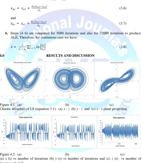
Figure 4.1. (a) (b) (c)
Chaotic attractors of LS (equation 3.1): (a) x - z (b) y - z and (c) x - y plane projection
Figure 4.2. (a) (b) (c)
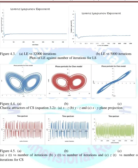
Lorenz Lyapunov Exponent
Lorenz Lyapunov Exponent
Figure 4.3. (a) LE vs 32000 iterations (b) LE vs 5000 iterations Plots of LE against number of iterations for LS
Figure 4.4. (a) (b) (c)
Chaotic attractors of CS (equation 3.2): (a) x - z (b) y - z and (c) x - y plane projection
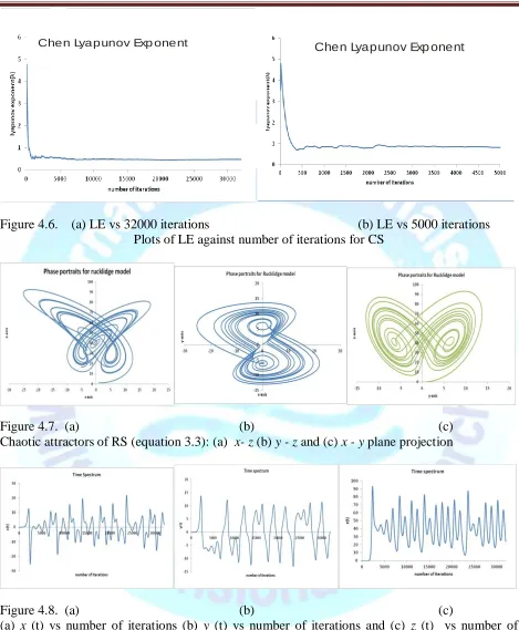
Figure 4.5. (a) (b) (c)
Chen Lyapunov Exp onent Chen Lyapunov Exp onent
Figure 4.6. (a) LE vs 32000 iterations (b) LE vs 5000 iterations Plots of LE against number of iterations for CS
Figure 4.7. (a) (b) (c)
Chaotic attractors of RS (equation 3.3): (a) x- z (b) y - z and (c) x - y plane projection
Figure 4.8. (a) (b) (c)
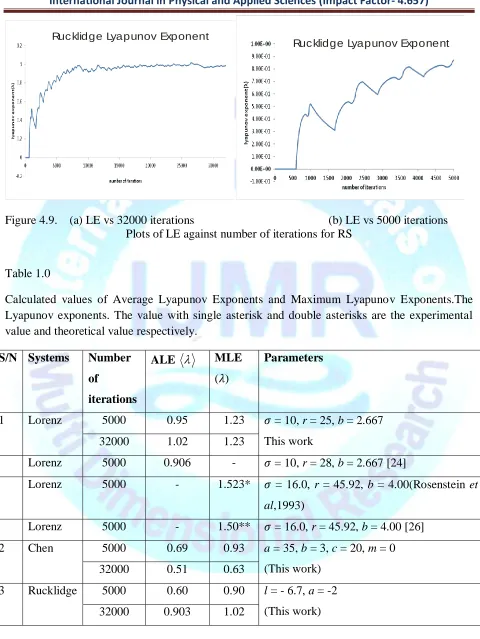
Rucklidge Lyapunov Exponent
Rucklidge Lyapunov Exponent
Figure 4.9. (a) LE vs 32000 iterations (b) LE vs 5000 iterations Plots of LE against number of iterations for RS
Table 1.0
Calculated values of Average Lyapunov Exponents and Maximum Lyapunov Exponents.The Lyapunov exponents. The value with single asterisk and double asterisks are the experimental value and theoretical value respectively.
S/N Systems Number of
iterations
ALE
MLE (𝜆)Parameters
1 Lorenz 5000 0.95 1.23 𝜎 = 10, r = 25, b = 2.667
This work
32000 1.02 1.23
Lorenz 5000 0.906 - 𝜎 = 10, r = 28, b = 2.667 [24]
Lorenz 5000 - 1.523* 𝜎 = 16.0, r = 45.92, b = 4.00(Rosenstein et
al,1993)
Lorenz 5000 - 1.50** 𝜎 = 16.0, r = 45.92, b = 4.00 [26]
2 Chen 5000 0.69 0.93 a = 35, b = 3, c = 20, m = 0
(This work)
32000 0.51 0.63
3 Rucklidge 5000 0.60 0.90 l = - 6.7, a = -2
(This work)
4.1 Discussion
The primary focus of this paper is to compute the MLE for the Lorenz-like systems (CS and RS) and also to characterize the Lorenz-like system. The system dynamics were studied with computer simulations. The solutions of the systems considered have a wide range of dynamical behaviour. The time series plot of the x-coordinate, y-coordinate and z-coordinate revealed that the systems are non-linear and signifies the existence of higher order periodicities. In this work it was observed that the LS is more chaotic than CS and RS but shared similar topological structure with them. All the systems can be characterized as dissipative chaotic with topological structure. The Lorenz and the Chen attractors have similar but different topological structures.
In figure 4.1(a – c) and 4.2(a – c) shows the trajectory of the LS. The fourth-order R-K algorithm was used with step height 0.0025. Figures 4.1(a – c) show the 2-dimensional Lorenz attractor and the projections on x-y, x-z and y-z planes in phase space of the portion of the trajectory corresponding to 32000 iterations. The orbits seem to be highly predictable but when the orbits reach the mid-region, a chaotic mixing occurs. Figures 4.2(a – c) shows the correlation between the time variable tand the function x(t), y (t) and z (t) respectively. It can be seen that as t tends to infinity the dynamical behaviour of system (3.1) changes repeatedly, leading to complex dynamics such as bifurcation and chaos. The ALE
is estimated to be 0.95 and the MLE λ is 1.23 in figure 4.3 (b) when the number of iteration is5000 but when the number of iteration increases to 32000, the ALE
is 1.02 with MLE λ at 1.23 as obtained from figure 4.3(a). The ALE occurs at the same time for both iterations (i.e. 5000 and 32000).Figures 4.4(a – c) and 4.5(a – c) shows the 2-dimensional Chen attractor and the projections on x-y, x-z and y-z planes in phase space of the portion of the trajectory corresponding to 32000 iterations. Figure 4.5(a – c) shows the correlation between the time variable tand the function x (t), y (t) and z (t) respectively. The ALE
is estimated to be 0.69 with MLE value of 0.93 for the 5000 iterations infigure 4.6(b) and when the number of iterations is 32000, the ALE
is 0.51 with its Maximum value of at 0.63 in figure 4.6(a).Figures 4.7(a – c) shows the 2-dimensional Rucklidge attractor and the projections on x-y, x-z and y-z planes in phase space of the portion of the trajectory corresponding to 32000 iterations. Figure 4.8 (a –c) shows the correlation between the time variable tand the function x (t), y (t) and z (t) respectively. The ALE
is 0.6 and MLE λ is estimated to be 0.90 at 5000 iterations in figure 4.9(b). When the numberof iterations is increased to 32000, the ALE
is 0.903 while the MLE λ is 1.02 in figure 4.9(a).5.0 CONCLUSION
chaotic and the long-term future evolution of these systems can't be predicted except to within certain size of the attractor.
REFERENCES
[1]Bailey .B. A., Ellner .S. and Nychka .D.W. (1991). Chaos with Confidence: Asymptotics and Applications of Local Lyapunov
Exponents.American MathematicalSociety.Biomathematics graduate program Department of statistics. North Carolina State University, Raleigh, NC 27695-8203.
[2]Barnett .W. A., Gallant .A. R., Hinich .M.J., Jungeilges .J. A., Kaplan .D. T. and Jensen .M. J. (1997). A Single-Blind Controlled
Competition Among Tests for Nonlinearity and Chaos. Journal of Econometrics.82, 157-162.
[3]C elikovsky .S. and Chen .G. (2002). On A Generalized Lorenz Canonical Form of Chaotic Systems. Int. J. Bifurcation and Chaos. 12. 1789-1812.
[4] C elikovsky .S. and Chen .G. (2003). Hyperbolic-type generalized Lorenz Chaotic System and its Canonical form. Proc. 15th IFAC Triennial World Congress on Automatic Control (IFAC'02); Barcelona, Spain.22-27.
[5]Chen .G. and L𝑢 .J. (2003). Dynamical Analysis,Control and Synchronization of the Generalized Lorenz Systems Family (in Chinese). Beijing: Science Press.
[6]Chen .G. and Ueta .T. (1999). Yet Another Chaotic Attractor. Int. J. Bifurcation and Chaos. 9. 465 1466.
[7]Christopher .L. W.and Roger .M. S. (2007). An Efficient method For RecoveringLyapunov Vectors From Singular Vectors. Tellus A. 59 (3). 355-366. DOI: 10.1111/j.1600-870.2007.00234.
[8]Dechert .W.D and Gencay .R. (1992). Lyapunov Exponents as a Nonparametric Diagnostic for Stability Analysis.Jounal of Applied Econometrics. 7. S41-S60.
[9]Deng .B. (1995). Constructing Lorenz type Attractors through Singular Perturbations. Int. J. Bifurcation and Chaos. 5. 1633-1642.
[10]Ershov .S.V., Alexei .B. and Potapov .K. (1998).On the Concept of Stationary Lyapunov Basis. Elsevier Physica D. 118. 167-198.
[11]Fernández-Rodríguez .F.,Sosvilla-Rivero .S. and Andrada-Félix .J. (2003). A New Test for Chaotic Dynamics Using Lyapunov Exponent.Documento de Trabajo 09. FEDEA (available at ftp://ftp.fedea.es/pub/Papers/2000/dt2003-09.pdf)
[12]Gleison .F.V.A., Christopher .L. and Luis .A .A. (2006). Piecewise Affine Models of Chaotic Attractos: The Rossler and Lorenz System. Chaos: An Interdisciplinary Journal of Non Linear Science. 16. Issue 1, 013115; http://dx.doi.org/10.1063/1.2149527.
[13]Hou. Z. T., Kang .N, Kong .X. X., Chen .G. R and Yan .G. J. (2010). Bifurcat.Chaos.Int. J. Bifurcat.Chaos.20. 557
[14]Kottos .T. Izrailev .F.M. and Politi .A. (1999). Finite-length Lyapunov exponents and conductance for quasi-1D disordered solids. Physica D. 131.155–169.
[15]L𝑢 .J, Chen.G. and Cheng .D. (2004). A New Chaotic System and Beyond: The Generalized Lorenz-Like System. International Journal of Bifurcation and Chaos.World Scientific Publishing Company. 14. 5. 1507-1537.
[17]Rosenstein .M. T., Collins .J. J. and Carlo .J. D. (1992). A Practical Method for Calculating Largest Lyapunov Exponents from Small Data Sets.NeuroMuscular Research Center and Department of Biomedical Engineering, Boston University, 44 Cummington Street, Boston, MA 02215,USA.
[18]Rosenstein .M. T., Collins .J. J. and Carlo .J. D. (1993). A practical method for calculating largest Lyapunov exponents from small data sets. Physica D. 65, 117-126.
[19]Rucklidge .A. M. (1992). Chaos In Models of Double Convection. J. Fluid Mech. 237. 209-229. [20]Ruth .S., Ying-Chemg .L. and Qingfei .C. (2008). Characterization of Non stationary Chaotic Systems.Physical Review E77.026208.doi:10.1103/Phyreve.77.026 208.Pacs Number(S): 05.45._a [21]Salau .T. A. and Ajide .O.O. (2012).Simulation and Lyapunov’s Exponents Characterisation of Lorenz and Rösler Dynamics.International Journal of Engineering and Technology. 2(9) 1543-1544 ISSN: 2049-2060.
[22]Sprott .J. C. (1997). Simplest Dissipative Chaotic Flow.Phys. Lett. A. 228. 271-274. [23]Sprott .J. C. (2003). Chaos And Time-Series Analysis. Oxford: Oxford University Press.
[24]Tufillaro .N. B., Abbott .T. and Reilly .J. (1992).An Experimental Approach to Nonlinear Dynamics and Chaos.Addison–Wesley.
[25]Vane ce k .A. and C elikovsky .S. (1996). Control Systems: From Linear Analysis to Synthesis of Chaos. London: Prentice-Hall.