The relevance of foreshocks in earthquake triggering: A statistical study

1

The

relevance

of

foreshocks

in

earthquake

triggering:

A

statistical

study

E.Lippiello1_,C.Godano1_{,L.deArcangelis}2

DepartmentofMathematicsandPhysics,UniversityofCampania“L.Vanvitelli”,VialeLincoln5,81100Caserta,Italy

2

Abstract

Anincreaseofseismicactivity isoftenobservedbeforelargeearthquakes. Events

responsi-bleforthisincreaseareusuallynamedforeshockandtheiroccurrenceprobablyrepresentsthe

mostreliableprecursorypattern. Manyforeshocksstatisticalfeatures canbe interpretedinterms

ofthestandardmainshock-to-aftershocktriggeringprocessandarerecovered intheEpidemic

TypeAftershock SequenceETASmodel. Herewepresentastatisticalstudy ofinstrumental

seismiccatalogsfromfourdifferent geographicregions. Wefocusonsomecommonfeatures

offoreshocksinthefourcatalogswhichcannotbereproducedbytheETASmodel. In

par-ticularwefind ininstrumentalcatalogsasignificantlylargernumberofforeshocksthanthe

onepredictedbytheETASmodel. Weshowthatthisforeshockexcesscannotbeattributed

tocatalog incompleteness.Wethereforeproposeageneralizedformulationof theETASmodel,

theETAFSmodel,whichexplicitlyincludesforeshockoccurrence. Statisticalfeaturesof

af-tershocksandforeshocksintheETAFS modelareinverygoodagreementwith

instrumen-talresults.

1 Introduction

Theepidemic-type-aftershocksequenceETASmodel Ogata[1985,1988a,b,1989]is

nowadaysconsidered“adefactostandardmodel,or nullhypotheses,for othermodelsand

ideastobecomparedto”Huangetal. [2016]The modelassumesthattwoclassesof

earth-quakesexist: Independentbackgroundandtriggeredearthquakes. Anepidemicorganization

ofeventsarisesundertheassumptionthat eachearthquakecantriggeritsowndescendents

lead-ingtoabranchingorganization. Fromaphysicalpointof view,backgroundseismicitycanbe

thoughtas theeffectoftheslowtectonic drivewhereastriggeredearthquakesareinducedby

stressredistributionafter previousshocks. Inthe ETASmodeltheoccurrencerateoftriggered

eventsisobtained onthebasisofwellestablishedempirical lawscontrollingthe spatio-temporal

clusteringofaftershocks. Asaconsequence,byconstruction,themodelisveryefficientin

re-producingstatistical featuresof aftershockorganizationobservedinexperimentalcatalogs. At

thesametime,intheETASmodelaneventcantriggeralsoalargershock.In thissituation

thetriggeringeventisoftennamed“foreshock”andthetriggeredearthquake,ifit isthelargest

eventinthesequence,isnamed“mainshock”.

Inthisstudyweadopt thestandarddefinition ofmainshocksaseventssufficiently

iso-latedintimeandspacefromotherlargerevents. Foreshocks(aftershocks)arethenallevents

theETASframework,thisclassificationof eventsdoes notreflectdifferentphysical

proper-tiessince,asanticipated, onlytwokinds (independentortriggered)earthquakesare assumed

and,for instance,amainshockcanbeeitheranindependent oratriggeredearthquake. On the

otherhand,accordingtoanucleation theoryOhnaka[1992,1993];Dodgeetal.[1996],the

nucleationphasecanbecharacterizedbythe occurrenceof smallerearthquakesinsidethe

re-gioninvolved inthefracture processofthesubsequent incominglargershock.Thispre-shock

seismicityisnotimplementedintheETASmodel andthemainquestionaddressedinthisstudy

isifitsinclusion,within theETASmodeling,givesamoreaccuratedescriptionof offoreshock

organizationininstrumentalcatalogs. Inthe lastfiveyearsseveralstudieshaveshownalack

offoreshocksinETASwithrespecttoinstrumentalcatalogsBrodsky[2011];Lippielloetal.

[2012c];Shearer[2012a, b];Hainzl[2013];Shearer[2013];Bouchonetal. [2013];Mignan

[2014];ChenandShearer[2013];BrodskyandLay [2014];OgataandKatsura[2014];Felzer

etal. [2015];BouchonandMarsan [2015];deArcangelisetal.[2016];Lippielloetal. [2017].

Nevertheless,thedeficit offoreshocksinETAScatalogshasbeenattributed,atleastpartially,

tothe deficitofaftershocksininstrumentalcatalogscausedbyspuriousincompleteness. This

pointwillbediscussedinthefollowingsectionswherewe provideevidencethatit cannot

jus-tifytheexcessofforeshocksininstrumentaldatasets.

2 Datasetsanddefinitions

Weperformasystematicanalysisof fourdifferentinstrumentalcatalogs: Therelocated

SouthernCaliforniaearthquake catalog(RSCEC)Haukssonetal. [2012](from01/01/1981to

12/31/2013),therelocatedNorthernCaliforniaearthquakecatalog (RNCEC)Waldhauserand

Schaff [2008](from01/01/1981to06/30/2011),theItalian earthquakecatalog(ItEC)[ISI](from

01/01/2002to12/31/2012) andtheJapaneseearthquake catalog(JaEC)[NIE](from01/01/1966

to01/30/2011). Weusethesamedefinition ofmainshock, aftershocksandforeshocksadopted

inLippielloetal.[2017].More precisely,we defineaneventas “mainshock”ifalarger

earth-quakedoes notoccurinthepreviousy daysandwithinadistanceL.In additionalarger

earth-quakemustnotoccur intheselected areainthefollowingy2 days. Wethenassociatetoeach

mainshockitsown“aftershocks”and“foreshocks”definedasallearthquakesrecorded inthe

subsequentor intheprecedingtimeintervalT = 12h, respectively,andwithinacircle of

radiusR≤RM centeredinthe mainshockepicenter. Weusedifferent RM for different

cat-alogs:RM = 2 kmforRSCEC andRNEC,RM = 5kmfor ItECandRM = 10km for

Oncemainshocksareidentified,they aregroupedinclassesaccordingtotheir

magni-tudem∈[mM,mM+1)and, foreachcatalog,we evaluatethetotalnumberof mainshocks

belongingtothegivenclassnmain(mM),thetotalnumberofassociatedaftershocksnaf t(mM)

andforeshocksnf ore(mM). Wealsoevaluatethe epicentraldistance∆rbetweeneach

main-aftershockandmain-foreshockcoupleandconstructtheaftershockandforeshockepicentral

distancedistributions,ρa(∆r,mM)andρf(∆r,mM).Their precisedefinitionisgiveninSec.4.1.

Thechoiceofparametershasbeendeeplyinvestigatedinpreviousstudies[Felzerand

Brodsky,2006;Lippielloetal.,2009a,2012c, 2017]andhereweimplementtypicalvalues,

L = 100km,y = 3 andy2 = 0.5. Thevalueof RM isfixedimposingthat, foreach

in-strumentalcatalog,differentchoicesofT ≤12hproducessimilarresultsρa(∆r,mM)when

∆r <RM.ThisleadstoRM =2,2,5,10km,forRSCEC,NSCEC; ItECandJMAC,

re-spectively.

2.1 The ETAS model

The ETAS model is specified by the conditional intensity function, which represents the

expected seismicity rate in a given space position conditioned to a given observational history.

The conditional intensity functionΛ(m, ~x, t), which represents the occurrence probability of

events with magnitudem≥mc in the position~xat timet, can be written in the following

form:

Λ(m, ~r, t) = [µw(~r) +Q(|~ri−~r|, t−ti, mi)]

1 blog(10)10

−b(m−mc) ₍₁₎

and

Q(∆ri, t−ti, mi) =

A(p−1) c

X

i:ti<t

10α(mi−mc)

1 +t−ti c

−p

G(∆ri, mi) (2)

where∆ri = |~ri −~r|and the sum extends over all events with magnitudemi, epicentral

coordinates~xi and occurrence timeti< t. The functionG(∆ri, mi)is a spatial kernel which

explicitly depends on the triggering magnitudemi andµw(~x)is a time independent

contri-bution due to background seismicity. The form of the spatio-temporal kernel (Eq.(2)

imple-ments three well established laws for aftershock triggering:

• A1: The number of aftershocksn_a depends on the mainshock magnitude class,

accord-ing to the productivity lawna=Ka10αamM;

• A2: The aftershock number decays as function of the time from the mainshock,

con-sistently with the Omori lawna(∆t)∼∆t−p withp≃0.8;

• A3: The linear density distribution of epicentral distances between mainshock and

af-tershocks (∆r) clearly depends on the mainshock magnitude classmM with the

aver-age distanceL(mM)∝10γmM withγ≃0.4.

In the following we present results from numerical simulations of the ETAS model

per-formed according to the algorithm discussed in ref.Lippiello et al.[2012c, 2017]; de

Ar-cangelis et al.[2016, 2018]. In particular, the spatial functionw(~x)is obtained from

the smoothed seismicity whereas the functional form ofG(∆ri, mi)is tuned in order

to collpase the aftershock epicentral distribution on the instrumental one, for all

val-ues ofmM.

3 Results

3.1 Previous Results

The statistical features of foreshocks in instrumental catalogs has been recently

inves-tigated in ref.Lippiello et al.[2017]. This study has shown that foreshocks follow

em-pirical laws like (A1-A3) of aftershocks but with important differences. More precisely:

• F1: The number of foreshocksn_f depends on the mainshock magnitude class

accord-ing to a productivity lawnf =Kf10αfmM;

• F1b: The number of foreshocks is systematically smaller than the aftershock number

andαf ≃0.7αa;

• F2: The foreshock number increases approaching the mainshock occurrence time,

con-sistently with an inverse Omori lawnf(∆t)∼ |∆t|−p withp≃0.8;

• F3: The linear density distribution of epicentral distances fore-mainshockρ_f(∆r, m_M)

depends on the mainshock magnitude class with a roughly symmetrical behavior

be-tween spatial distribution before and after the mainshocksρf(∆r, mM)≃ρa(∆r, mM);

• F3b: The foreshock linear density distributionρ_f(∆r, m_M)does not depend on the value

of the lower magnitude cut-offmth.

The comparison between instrumental and ETAS catalogs has shown (Lippiello et al.[2017])

that it is possible to generate ETAS catalogs which reproduce at quantitative level the

statis-tical features (A1-A3) of instrumental aftershocks. At the same time ETAS catalogs can

re-produce foreshock features F1 and F2. Conversely it is not possible to generate ETAS

cata-logs with foreshocks obeying features F3 and F3b. Furthermore, ETAS catacata-logs always present

a deficit of foreshocks with respect to instrumental catalogs. In the following section we will

3.2 The aftershock and foreshock number

In Fig.1 we plot the ratio between aftershock and mainshock numbernaf t(mM)/nmain(mM)

for different mainshock classesmM and for the different instrumental catalogs. We also plot

the ratio between foreshock and mainshock numbernf ore(mM)/nmain(mM). We only

con-sider events with magnitudem > mth = 2. The lower thresholdmth must not be confused

withmc in Eq.(2). Indeed,mc is a fixed parameter of the ETAS model and synthetic catalogs

contain only events withm≥mc. The lower magnitudemth, conversely, is a parameter

im-plemented in the data analysis and it can be arbitrarily varied withmth≥mc.

Results in Fig.1 show that the aftershock number is systematically larger than the

fore-shock number and this difference increases for increasingmM. The aftershock number is

con-sistent with the Utsu-productivity law (A1)

naf t(mM)/nmain(mM) =Ka10αmM (3)

and a similar law is also observed for foreshocksnf ore(mM)/nmain(mM) = Kf10αfmM

(F1).

In Fig.1 we compare results fornaf t(mM)/nmain(mM)andnf ore(mM)/nmain(mM)

for the RSCEC with the results obtained applying the same definition of aftershocks,

main-shocks and foremain-shocks to simulated ETAS catalogs. The values of bothnaf t(mM)/nmain(mM)

andnf ore(mM)/nmain(mM)depend on the parametersA, p, c, α(Eq.(2) of the numerical model.

In particular, in first approximation the value ofnaf t(mM)/nmain(mM)is given by

naf t(mM)≃µ(RM)T+nmain(mM)BR10α(mM−mc) 1−(T /c+ 1)1−pH(Rm). (4)

In this equationµ(RM)is the average background rate inside a circle of radiusRM,nmain(m)dm

represents the number of mainshocks in the range[m, m+dm),BR = _log(10)(Ab−α) is the branching ratio, i.e. the average number of events triggered by any earthquake, andH(Rm) =

RRm

0 d∆rG(∆r, mM). Neglecting the background contribution, Eq.(4) indicates that the ETAS model can reproduce the experimental result Eq.(3) withαf =α. In numerical simulations

we have explored a wide range of ETAS parametersA, p, c, αand verified that there exists a

set of parameters leading to ETAS catalogs with the same behavior ofnaf t(mM)/nmain(mM)

of the instrumental ones. In all cases the agreement between ETAS and instrumental catalogs

is always recovered for values ofα&αf. We wish to stress the difference between αand

αf: αis the model parameter which controls the productivity law in numerical simulations

whereasαf is the value obtained applying our definition of mainshock and aftershock to ETAS

catalogsandthenperformingafitaccordingtoEq.(3).Thesmall discrepanciesbetweenαand

αf canbeattributedtothe backgroundcontributionwhichweaklyaffectsdataatsmallmM

whereasitcanbeneglectedforincreasing mM.

Acentralobservationisthat allchoicesof parametersproducingagreementinnaf t(mM)/nmain(mM)

betweenETASandinstrumentalcatalogsgiveavalueof nf ore(mM)/nmain(mM)inETAS

catalogssystematicallysmallerthantheinstrumentalvalue. Itisdifficulttoobtainasimple

approximatedexpressionfortheforeshocknumberasfunctionofmM asinEq.(4).However,

itisreasonabletoexpectthat therationaf t(mM)/nf ore(mM)weaklydependsonmodel

pa-rameters. Thisissupportedbynumericalsimulationswherewe fixαinordertohavethesame

valueofαf inETAScatalogs. ResultsplottedinFig.(2)showthatdifferentchoicesof B,p,c

leadtosimilarresultsfornaf t(mM)/nf ore(mM),significantlylargerthanthe experimental

valueforany mM.

4 CatalogincompletenessandtheETASI2model

Asanticipatedinthe introduction,the incompletenessofinstrumentaldatasetscanbe

responsibleforthe observeddifferenceswithETAScatalogs.Indeed, becauseofthe overlap

ofseismiccodawaves, manyaftershocksarenotrecordedinparticularinthefirsttemporal

periodsafterlargeshocksKagan[2004];Helmstetteretal.[2006];Enescuetal.[2007];Peng

etal. [2007];PengandZhao[2009];OmiandAihara [2013];Lippielloetal.[2016];Hainzl

[2016a,b];deArcangelisetal.[2018]. Thedirectinspectionof seismicsignals[Lippielloetal.,

2016;deArcangelisetal.,2018]hasshownthat, atatemporaldistanceτ after aneventof

mag-nitudem0,thereexistsalowermagnitudelevelmx(τ,m0)such thatitisimpossibleto

de-tecteventswithm≤mx(τ,m0).Resultsindicate alogarithmicdecayofmx(τ,m0)intime

mx(τ, m0) =m0−φlog(τ)−∆m (5)

withφ≃1 and∆m≃1, ifτ is measured in seconds. Accordingly earthquakes can be

hid-den by larger events occurring before them at small temporal distances. As a consequence

in-completeness affects more strongly the aftershock than the foreshock number and could

pro-vide an explanation for the larger value ofnf ore(mM)/naf t(mM)in instrumental catalogs.

In the following we take explicitly into account the aftershock incompleteness adopting

the same procedure developed in ref.de Arcangelis et al.[2018] to reproduce both the non-trivial

dependence of thec-value in the OU law on the manishock magnitudeShcherbakov et al.[2005];

David-senandBaiesi[2016],aswellasthenon trivialmagnitudecorrelationsbetweensubsequent

earthquakesLippielloetal. [2007b,2008,2009b,a];Sarlisetal. [2010a,b];Sarlis[2011];

Lip-pielloetal.[2012b, 2013].Themodel,definedas ETASI2model,implementsaftershock

in-completenessbymultiplyingtheoccurrencerateQ(∆r,t−ti,mi)inEq.(2)byadetection

ratefunctionofthe magnitudeΦ(m|q,σ)representedbythecumulativedistributionfunction

ofthenormal distribution. ThefunctionΦ(m|q,σ)dependsontwoparametersqandσ

rep-resenting,respectively, themagnitudewitha50% detectionrate andapartiallydetected

mag-nituderange. Inotherwords,Φ(q|q,σ) = 0.5 whereasΦ(m|q,σ) ≃ 0 whenm < q−σ

andΦ(m|q,σ) ≃ 1when m > q−σ.In theETASI2 modeltheqparameterdependson

timeaccordingtoEq.(5),q=mx(τ,mi).

Wehaveperformedextendednumericalsimulationsof theETASI2 modelexploringa

widerangeofmodel parametersandevaluatednaf t(mM)andnf ore(mM).Restrictingto

pa-rameterswithnaf t(mM)/nmain(mM)inagreementwiththeinstrumentalRSCECcatalog,

wefind(Fig.(2))that, asexpected,theincompletenessincreasesthevalueofnf ore(mM)/naf t(mM)

which,however,stillremainssystematicallysmallerthanthevaluefoundininstrumental

cat-alogs. Forfixedφand∆minEq.(5),theratio nf ore(mM)/naf t(mM)does notstrongly

de-pendondifferentchoicesofσ,aswellasondifferentvaluesof A,p,candisalways

signif-icantsmallerthanthenumericalone. Wealsofind thatnf ore(mM)/naf t(mM)slightly

in-creasesfordecreasing∆mandbecomes approximately∆mindependent for∆m.0.

How-ever,alsointhiscasethevaluenf ore(mM)/naf t(mM)issignificantlysmallerthantheone

measuredintheinstrumentalcatalogs.Theoriginof thisdiscrepancyisthat incompleteness

alsoaffectsthe foreshocknumber. Indeed,consideringamainshockof magnitudem2 triggered

byanevent(aforeshock)withmagnitudem1 < m2,incompletenessdoes notonlyaffect

theidentificationofbothm1 andm2 butitcanhideforeshockswithmagnitudem < m1

occurringbetweenthem.Therefore,iftheparametersaretunedinordertoproduceahigher

aftershockincompletenessthisalsoreducesthe foreshocknumberandtheexperimentalresult

isneverrecovered. In Fig.1weplot foreachinstrumentalcatalogtheresultsof theETASI2

modelsettingthemodel parametersinordertoachievethebestagreementfor naf t(mM)/nmain(mM)

and minimizing the discrepancy fornf ore(mM)/nmain(mM). Results are obtained

assum-ingφ = 0.75and∆m = 0.8for all catalogs, and keepingσ = 0.3. Furthermore we use

p= 1.2 andc = 0.01sec. The values ofAandαproducing the best agreement are listed

in the caption of Fig.1.

4.1 Aftershock and Foreshock spatial distribution

In the previous section we have shown that incompleteness can only partially explain

the deficit of foreshocks in ETAS catalogs. As discussed in Sec.3.1 an important difference,

which has been observed in previous studies concerns the feature F2. This implies that even

if the aftershock and foreshock number are different, their linear density distribution are

sim-ilarρa(∆r, mM)≃ρf(∆r, mM)for different values ofmM.

Inthisstudywefocusontheaftershockandforeshockaverageepicentraldistanceζa(∆r,mM)

andζb(∆r, mM)defined as ζa(∆r, mM)≡ ∆1r

R∆r

0 dxrρa(r,mM)andζf(∆r,mM)≡1∆r

R∆r

0 drrρa(r,mM).

Hereρa(∆r, mM)is the aftershock linear density distribution defined as the number of

after-shocks with epicentral distance from the mainshock in the interval[∆r,1.2∆r), divided by

0.2∆rand by the total number of aftershocks in the interval[0, R]. A similar definition

ap-plies to the foreshock linear densityρf(∆r, mM).

In Fig.(3) we plotζa(∆r, mM)andζf(∆r, mM)for different catalogs. It is evident that,

for all catalogs, data corresponding to differentmM are well separated and in all casesζa(∆r, mM)≃

ζf(∆r, mM). The latter result is a direct consequence of the similarityρa(∆r, mM)≃ρf(∆r, mM)

(F2) which cannot be reproduced by the ETAS model. Indeed, neglecting the contribution of

background seismicity, we indicate bypa(m|m0)the probability that an event with magnitude

m0 triggers a smaller earthquake (m < m0) inside a temporal windowT. The aftershock

epicentral distribution is approximatively given byρa(∆r, m0)≃pa(m|m0)G(∆r, m0).

Con-sidering triggering events in the range[mM, mM+dM)we therefore obtain

ρa(∆r, mM)≃

RmM+dM

mM dm0

Rm0

mthdmG(∆r, m0)pa(m|m0)

RmM+dM

mM dm0

Rm0

mthdmpa(m|m0)

. (6)

At the same time we indicate withpf(m|m0)the probability that an event with magnitudem

triggers a larger earthquake (m < m0) inside a temporal windowT. In this case, the

fore-shock epicentral distance is approximatively given byρf(∆r, m0) ≃ pf(m|m0)G(∆r, m)

and considering triggered events in the range[mM, mM+dM)we find

ρf(∆r, mM)≃

RmM+dM

mM dm0

Rm0

mthdmG(∆r, m)pf(m|m0)

RmM+dM

mM dm0

Rm0

mthdmpf(m|m0)

. (7)

We wish to stress the fundamental difference between Eq. (6) and Eq. (7). In Eq. (6) the

spa-tial distance is controlled by the kernelG(∆r, m0)which depends on m0 ∈ [mM, mM +

dM)and ifdM → 0ρa(∆r, mM) ≃ G(∆r, mM). Conversely, in Eq. (7) the spatial

ker-nel isG(∆r, m)withm ranging inm∈[mth, mM). In this case ifdM →0, sincepf(m|m0)

C

contributionfromm≃mth whichleadstoρf(∆r,mM)≃G(∆r,mth).Asaconsequence,

inthe ETASmodel,weexpectthatρf(∆r,mM)onlyweaklydependsonmM differentlyfrom

ρa and strongly depends on mth. The comparison between Eq.s(6,7) therefore shows that,

in-dependently of the value of the model parameters, the condition ρa(∆r,mM)≃ρf(∆r,mM)

can never be observed. This is confirmed by the results of numerical simulations (Fig.(4)) which show that, even if one can generate ETAS catalogs with ζa(∆r,mM)in good agreement with

instrumental catalogs ( Fig.(4)a), significant differences are observed between the numeric and the experimental ζf(∆r,mM)( Fig.(4)b). This difference becomes more pronounced for

in-creasing mM and can simply attributed to the nature of foreshocks in the ETAS model which

are tipical events that have triggered a larger shock.

Wefinallystress thattheobserveddifferenceinζf(∆r,mM)betweeninstrumentaland

ETAS catalogs cannot be related to catalog incompleteness. Indeed, incompleteness typically affects the number of aftershocks and foreshocks but not their spatial distribution. We have explicitly verified this point by means of numerical simulations evidencing that the dependence on ∆rand mM of ζa(∆r,mM)and ζf(∆r,mM)is substantially indistinguishable for the ETAS

andthe ETASI2model(notshown).

5 TheETAFSmodel

Accordingtothe nucleationtheory[Ohnaka,1992,1993;Dodgeetal.,1996]one

ex-pectsaconcentrationof seismicityinsidethenucleation zoneduringthepreparatoryphase.

Thiskindofseismicactivity isnotconsideredintheETASmodelandcanjustifytheexcess

offoreshocksobservedininstrumentalcatalogs(Fig.(2)). Furthermore,sincethesizeof the

nucleation zone scales with the magnitude of the incoming mainshock[Ohnaka, 1992; Dodge

etal., 1996], the pre-seismic activity can also explain the result ζa(∆r,mM)≃ζf(∆r,mM)

(Fig.(3)). We then propose a novel model, the Epidemic Type Aftershocks and Foreshock Se-quence (ETAFS) model, which implements together with the standard aftershock triggering

alsoadditionalearthquakescorrespondingtotheforeshocksexpectedaccordingtoanucleation

scenario.In theETAFSmodeleach earthquakecantriggeritsownaftershockswitha

prob-abilityQ(Eq.(2))as intheETASmodel. Thenewingredientisthateach earthquakecanbe

alsoanticipatedbyanumberofforeshocksaccordingtoaprobability

Qf(∆r, t−ti, mi) =

B(p−1) c′

X

i:ti<t

10α′_(m

i−mc)_{1 +}t−ti

c′

−p

Gf(∆ri, mi). (8)

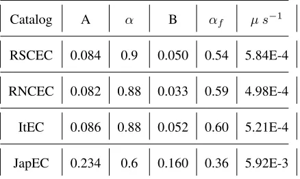
Table 1. Best parameters of the ETAFS model

Catalog A α B αf µ s−1

RSCEC 0.084 0.9 0.050 0.54 5.84E-4

RNCEC 0.082 0.88 0.033 0.59 4.98E-4

ItEC 0.086 0.88 0.052 0.60 5.21E-4

JapEC 0.234 0.6 0.160 0.36 5.92E-3

Because of the experimental resultρa(∆r, mM)≃ρf(∆r, mM)we setGf(∆ri, mi) =G(∆ri, mi)

in Eq.(2). We have also implemented an inverse-Omori law with the samepas for aftershock

occurrence, to reduce the number of model parameters. There is no physical justification for

it and we expect that similar results can be recovered with other functional forms of

tempo-ral clustering. We fixc= 100s and chose the parametersB, c′_{, α}′_{, for each instrumental} cat-alog, in order to reproduce the valuenf ore(mM)/nmain(mM), for differentmM (see Tab. 1).

We also take explicitly into account aftershock incompleteness, implemented as in the ETASI2

model, and finally generate synthetic catalogs with the same number ofnaf t(mM)/nmain(mM)

andnf ore(mM)/nmain(mM)of instrumental ones. Fig.2 shows that for all values of mM ETASI2

catalogs contains the same number of both aftershocks and foreshocks of instrumental data

sets. In (Fig.4) we compare the average fore-mainshock distanceζf(∆r, mM)between the ETAFS

and the RSCEC catalog. Results show good agreement for all values ofmM.

6 Conclusions

In conclusions, we have discussed the differences between statistical features of

fore-shocks in ETAS and instrumental catalogs. We have then introduced the novel ETAFS model

which explicitly implements foreshocks in the ETAS model and is able to reproduce the

en-tire ensemble of experimental observations. All properties investigated in this study are

ob-tained by means of a stacking procedure. An interesting point is the behavior expected

accord-ing to the ETAFS model for the seismic activity before a saccord-ingle large shock. The best-fit

pa-rameters of the ETAFS model (Tab.1) indicate a small coefficientαf ≃1.1in the foreshock

productivity law and accordingly the number of foreshock remains relatively small also

daybefore amagnitudem=7 mainshock,withinaradiusof 10km. Thissmallnumber

im-pliesthat,for asinglemainshock,foreshockactivity canatmostappearintheformof

iso-latedburstsnotleadingtoanevidentsystematicincreaseoftheseismicrate. Thisis

consis-tentwithexperimentalobservations,wheretheinverseOmori-law isobtainedonlyaftera

stack-ingprocedureandrarelyobservedinsideisolated sequences[Papadopoulosetal.,2010;Daskalaki

etal.,2016].

Theagreementwithexperimentaldatasuggeststhatthe ETAFSmodelcancontribute

toasignificantimprovement ofpre-seismicforecasting. Arigorousvalidation ofthispoint,

however,needstobetestedinprospectivetests. Unfortunately,amainlimitationof themodel

isthatitisnotimmediatelysuitable tobeimplementedinthiskindof analysis.Indeed, in

or-dertoforecast theoccurrenceofanearthquake,accordingtotheETAFSmodel itis

neces-sarytodistinguishforeshockfromnormalearthquake triggering.Anattemptinthisdirection

([Lippielloetal.,2012c]) multipliesthe ETASoccurrenceprobabilitybyanad-hocfunction,

givingdifferentweightstoaftershockandforeshockclustering. Thisproducessignificant gain

inthe retrospectiveforecasting ofm>6 earthquakes.The natureofforeshocksimplemented

inthe ETAFSmodelisconsistentwiththisapproachpromotingfurtherstudiesonthe

rele-vanceof foreshocksinseismicforecasting.

0,1 1

0,1 1

n

(m

M

)/n

main

(m

M

) & n

fore

(m

M

)/n

main

(m

M

)

0,1 1

2 2,5 3 3,5 4

m

M

0,1 1

RSCEC

RNCEC

ItEC

JapEC

Figure 1. (Color online) The rationaf t(mM)/nmain(mM)andnf ore(mM)/nmain(mM)in

instru-mental and synthetic catalogs. Different panels correspond to different instruinstru-mental catalogs. We use open

symbols fornaf t(mM)/nmain(mM)and filled symbols fornf ore(mM)/nmain(mM). Results from the

in-strumental data sets are indicated with black circles. Green triangles are results for the ETASI2 model and red

squares for the ETAFS model. The error bars (of the same size of symbols) in numerical catalogs represent

the standard deviation from100realization of synthetic catalogs. The best parameter of the ETAFS model are

listed in Tab.1 whereas for the ETASI2 model the best agreement is obtained withA = 0.084,α = 0.9and

µ = 5.8510−4_s−1_{for RSCEC,A = 0.082,α = 0.88andµ = 4.9810}−4_s−1_{for RNCEC,A = 0.082,}

2 2,5 3 3,5 4

m

0,1 1

n

(m

M

)/n

aft

(m

M

)

Figure 2. (Color online) The rationf ore(mM)/naf t(mM)in the RSCEC catalog (blue stars) is

com-pared with the value obtained in synthetic ETAS and ETASI2 and ETAFS catalog. The black open symbols

are results for the ETAS model for different choices of the parametersA ∈ [0.05,0.12],p ∈ [1.1,1.25]

andc ∈ _{[0.001,0.1]. The red filled symbols are results for the ETASI2 model implementing Eq.(5) with}

φ = 0.75and∆m = 0.8and for different choices of the parametersA ∈ _{[0.05,0.12],p} ∈ _{[1.1,1.25]and}

c ∈ _[0.001,0.1]. Green symbols correspond toA = 0.084,c = 0.01andp = 1.2used in Fig.1 for the

RSCEC catalog and considering different values ofφ,∆mandσ. The filled magenta up triangles are results

of the ETAFS model with the best set of parameters listed in Tab.1.

10-3 10-2 10-1 100

0,01 0,1 1

∆r (km)

ζ

(

∆

r,m

) &

ζ

(

∆

r,m

)

0,01 0,1 1 10

∆r (km)

10-3 10-2 10-1

m_M=2 m_M=3 m_M=4

RSCEC

RNCEC

ItEC

JapEC

Figure 3. (Color online) The average distanceζa(∆r, mM)of aftershocks (open symbols) and of

fore-shocksζf(∆r, mM)(filled symbols) is plotted as function of∆rfor the different catalogs. Different

main-shock magnitude classes are plotted with different colors and symbols.

Acknowledgments

We thank the National Research Institute for Earth Science and Disaster Prevention for the

main-land Japan catalog.

References

From I.S.I.D.E. italian seismological instrumental and parametric data-base.

From Japan Meteorological Agency Earthquake Catalog, provided by N.I.E.D.

Bottiglieri, M., L. de Arcangelis, C. Godano, and E. Lippiello, The generalized omori law:

magnitude incompleteness or magnitude clustering,International Journal of Modern

Physics B,23(28n29), 5597–5608, doi:10.1142/S0217979209063882, 2009a.

Bottiglieri, M., E. Lippiello, C. Godano, and L. de Arcangelis, Identification and

spa-tiotemporal organization of aftershocks,Journal of Geophysical Research: Solid Earth,

114(B3), B03,303, doi:10.1029/2008JB005941, 2009b.

Bottiglieri, M., L. de Arcangelis, C. Godano, and E. Lippiello, Multiple-time scaling and

0,01 0,1 1

∆

r (km)

0,001 0,01 0,1 1

ζ

(

∆

r,m

M

)

m_M=2 m_M=3 m_M=4

0,01 0,1 1

∆

r (km)

0,01 0,1

ζ

(

∆

r,m

M

)

(a)

_(b)

Figure 4. (Color online) (Left panel) The average distance of aftershocksζa(∆r, mM)in the RSCEC

(open symbols) and in the synthetic ETASI2 catalogs (continuous lines) is plotted as function of∆rfor

dif-ferent mainshock magnitude classes. (Right Panel) The average distance of foreshocksζf(∆r, mM)in the

RSCEC (filled symbols) and in the synthetic ETASI2 catalog (continuous lines) is plotted as function of∆r

for different mainshock magnitude classes. Results for the EATFS model, for the best set of model parameters

listed in Tab.1, are plotted with crosses.

158,501, doi:10.1103/PhysRevLett.104.158501, 2010.

Bottiglieri, M., E. Lippiello, C. Godano, and L. de Arcangelis, Comparison of branching

models for seismicity and likelihood maximization through simulated annealing,Journal

of Geophysical Research: Solid Earth,116(B2), n/a–n/a, doi:10.1029/2009JB007060,

b02303, 2011.

Bouchon, M., and D. Marsan, Reply to artificial seismic acceleration,Nature Geosci.,8,

83, 2015.

Bouchon, M., V. Durand, D. Marsan, H. Karabulut, and J. Schmittbuhl, The long

precur-sory phase of most large interplate earthquakes,Nature Geosci.,6, 299302, 2013.

Brodsky, E. E., The spatial density of foreshocks,Geophysical Research Letters,38(10),

L10,305, doi:10.1029/2011GL047253, l10305, 2011.

Brodsky, E. E., and T. Lay, Recognizing foreshocks from the 1 april 2014 chile

earth-quake,Science,344(6185), 700–702, 2014.

Chen, X. W., and P. M. Shearer, California foreshock sequences suggest aseismic

trigger-ing process,Geophysical Research Letters,40(11), 2602–2607, doi:10.1002/grl.50444,

n/a, 2013.

Daskalaki, E., K. Spiliotis, C. Siettos, G. Minadakis, and G. A. Papadopoulos, Foreshocks

and short-term hazard assessment to large earthquakes using complex networks: the

case of the 2009 l’aquila earthquake,Nonlinear Processes in Geophysics Discussions,

2016, 1–20, doi:10.5194/npg-2015-80, 2016.

Davidsen, J., and M. Baiesi, Self-similar aftershock rates,Phys. Rev. E,94, 022,314, doi:

10.1103/PhysRevE.94.022314, 2016.

de Arcangelis, L., C. Godano, J. R. Grasso, and E. Lippiello, Statistical physics

ap-proach to earthquake occurrence and forecasting,Physics Reports,628, 1 – 91, doi:

http://dx.doi.org/10.1016/j.physrep.2016.03.002, statistical physics approach to

earth-quake occurrence and forecasting, 2016.

de Arcangelis, L., C. Godano, and E. Lippiello, The overlap of aftershock coda waves

and short-term postseismic forecasting,Journal of Geophysical Research: Solid Earth,

123(7), 5661–5674, doi:10.1029/2018JB015518, 2018.

Dodge, D. A., G. C. Beroza, and W. L. Ellsworth, Detailed observations of california

foreshock sequences: Implications for the earthquake initiation process,Journal of

Geophysical Research: Solid Earth,101(B10), 22,371–22,392, doi:10.1029/96JB02269,

Enescu, B., J. Mori, and M. Miyazawa, Quantifying early aftershock activity of the 2004

mid-niigata prefecture earthquake (mw6.6),Journal of Geophysical Research: Solid

Earth,112(B4), B04,310, doi:10.1029/2006JB004629, 2007.

Felzer, K. R., and E. E. Brodsky, Decay of aftershock density with distance indicates

triggering by dynamic stress,Nature,441, 735–738, 2006.

Felzer, K. R., M. T. Page, and A. J. Michael, Artificial seismic acceleration,Nature

Geosci.,8, 82–83, 2015.

Hainzl, S., Comment on self-similar earthquake triggering, bth’s law, and

fore-shock/aftershock magnitudes: Simulations, theory, and results forsouthern california

by p. m. shearer,Journal of Geophysical Research: Solid Earth,118(3), 1188–1191,

doi:10.1002/jgrb.50132, 2013.

Hainzl, S., Apparent triggering function of aftershocks resulting from rate-dependent

in-completeness of earthquake catalogs,Journal of Geophysical Research: Solid Earth,

121(9), 6499–6509, doi:10.1002/2016JB013319, 2016JB013319, 2016a.

Hainzl, S., Ratedependent incompleteness of earthquake catalogs,Seismological Research

Letters,87(2A), 337–344, 2016b.

Hauksson, E., P. Shearer, , and W. Yang, Waveform relocated earthquake catalog for

southern california (1981 to june 2011),Bulletin of the Seismological Society of America,

102(5), 2239–2244, doi:10.1785/0120120010, 2012.

Helmstetter, A., Y. Y. Kagan, and D. D. Jackson, Comparison of short-term and

time-independent earthquake forecast models for southern california,Bulletin of the

Seismo-logical Society of America,96(1), 90–106, doi:10.1785/0120050067, 2006.

Huang, Q., M. Gerstenberger, and J. Zhuang, Current challenges in statistical seismology,

Pure and Applied Geophysics,173(1), 1–3, doi:10.1007/s00024-015-1222-7, 2016.

Kagan, Y. Y., Short-term properties of earthquake catalogs and models of earthquake

source,Bulletin of the Seismological Society of America,94(4), 1207–1228, 2004.

Lippiello, E., M. Bottiglieri, C. Godano, and L. de Arcangelis, Dynamical scaling

and generalized omori law,Geophysical Research Letters,34(23), L23,301, doi:

10.1029/2007GL030963, 2007a.

Lippiello, E., C. Godano, and L. de Arcangelis, Dynamical scaling in branching models

for seismicity,Phys. Rev. Lett.,98, 098,501, doi:10.1103/PhysRevLett.98.098501, 2007b.

Lippiello, E., L. de Arcangelis, and C. Godano, Influence of time and space

correlations on earthquake magnitude,Phys. Rev. Lett.,100, 038,501, doi:

10.1103/PhysRevLett.100.038501, 2008.

Lippiello, E., L. de Arcangelis, and C. Godano, Role of static stress diffusion in the

spatiotemporal organization of aftershocks,Phys. Rev. Lett.,103, 038,501, doi:

10.1103/PhysRevLett.103.038501, 2009a.

Lippiello, E., L. de Arcangelis, and C. Godano, Time, space and magnitude correlations

in earthquake occurrence,International Journal of Modern Physics B,23(28n29), 5583–

5596, doi:10.1142/S0217979209063870, 2009b.

Lippiello, E., A. Corral, M. Bottiglieri, C. Godano, and L. de Arcangelis, Scaling behavior

of the earthquake intertime distribution: Influence of large shocks and time scales in the

omori law,Phys. Rev. E,86, 066,119, doi:10.1103/PhysRevE.86.066119, 2012a.

Lippiello, E., C. Godano, and L. de Arcangelis, The earthquake magnitude is

influ-enced by previous seismicity,Geophysical Research Letters,39(5), L05,309, doi:

10.1029/2012GL051083, 2012b.

Lippiello, E., W. Marzocchi, L. de Arcangelis, and C. Godano, Spatial organization of

foreshocks as a tool to forecast large earthquakes,Sci. Rep.,2, 1–6, 2012c.

Lippiello, E., C. Godano, and L. de Arcangelis, Magnitude correlations in the

Olami-Feder-Christensen model,Europhysics Letters,102(5), 59,002, 2013.

Lippiello, E., A. Cirillo, G. Godano, E. Papadimitriou, and V. Karakostas, Real-time

fore-cast of aftershocks from a single seismic station signal,Geophysical Research Letters,

43(12), 6252–6258, doi:10.1002/2016GL069748, 2016GL069748, 2016.

Lippiello, E., F. Giacco, W. Marzocchi, C. Godano, and L. d. Arcangelis, Statistical

fea-tures of foreshocks in instrumental and etas catalogs,Pure and Applied Geophysics, pp.

1–19, doi:10.1007/s00024-017-1502-5, 2017.

Mignan, A., The debate on the prognostic value of earthquake foreshocks: A

meta-analysis,Sci. Rep.,4, 4099–4103, 2014.

Ogata, Y., Statistical models for earthquake occurrences and residual analysis for point

processes,Research Memo. Technical report Inst. Statist. Math., Tokyo.,288, 1985.

Ogata, Y., Statistical models for earthquake occurrences and residual analysis for point

processes,J. Amer. Statist. Assoc.,83, 9 27, 1988a.

Ogata, Y., Space-time point-process models for earthquake occurrences,Ann. Inst.

Math.Statist.,50, 379402, 1988b.

Ogata, Y., A monte carlo method for high dimensional integration,Numerische

Ogata, Y., and K. Katsura, Comparing foreshock characteristics and foreshock forecasting

in observed and simulated earthquake catalogs,Journal of Geophysical Research: Solid

Earth,119(11), 8457–8477, doi:10.1002/2014JB011250, 2014JB011250, 2014.

Ohnaka, M., Earthquake source nucleation: A physical model for short-term precursors,

Tectonophysics,211(14), 149 – 178, 1992.

Ohnaka, M., Critical size of the nucleation zone of earthquake rupture inferred from

immediate foreshock activity,Journal of Physics of the Earth,41(1), 45–56, doi:

10.4294/jpe1952.41.45, 1993.

Omi, Y. O. Y. H., T., and K. Aihara, Forecasting large aftershocks within one day after

the main shock,Scientific Report,3(2218), 2013.

Papadopoulos, G. A., M. Charalampakis, A. Fokaefs, and G. Minadakis, Strong

fore-shock signal preceding the l’aquila (italy) earthquake (mw 6.3) of 6 april 2009,Natural

Hazards and Earth System Science,10(1), 19–24, doi:10.5194/nhess-10-19-2010, 2010.

Peng, Z., and P. Zhao, Migration of early aftershocks following the 2004 parkfield

earth-quake,Nature Geosci,2(12), 877–881, 2009.

Peng, Z., J. E. Vidale, M. Ishii, and A. Helmstetter, Seismicity rate immediately before

and after main shock rupture from high-frequency waveforms in japan,Journal of

Geo-physical Research: Solid Earth,112(B3), n/a–n/a, doi:10.1029/2006JB004386, b03306,

2007.

Sarlis, N. V., Magnitude correlations in global seismicity,Phys. Rev. E,84, 022,101, doi:

10.1103/PhysRevE.84.022101, 2011.

Sarlis, N. V., E. S. Skordas, and P. A. Varotsos, Nonextensivity and natural time: The case

of seismicity,Phys. Rev. E,82, 021,110, doi:10.1103/PhysRevE.82.021110, 2010a.

Sarlis, N. V., E. S. Skordas, and P. A. Varotsos, Nonextensivity and natural time: The case

of seismicity,Phys. Rev. E,82, 021,110, doi:10.1103/PhysRevE.82.021110, 2010b.

Shcherbakov, R., G. Yakovlev, D. L. Turcotte, and J. B. Rundle, Model for the

dis-tribution of aftershock interoccurrence times,Phys. Rev. Lett.,95, 218,501, doi:

10.1103/PhysRevLett.95.218501, 2005.

Shearer, P. M., Self-similar earthquake triggering, bath’s law, and foreshock/aftershock

magnitudes: Simulations, theory, and results for southern california,Journal of

Geophys-ical Research-Solid Earth,117, doi:10.1029/2011jb008957, n/a, 2012a.

Shearer, P. M., Space-time clustering of seismicity in california and the distance

2012b.

Shearer, P. M., Reply to comment by s. hainzl on self-similar earthquake triggering,

bth’s law, and foreshock/aftershock magnitudes: Simulations, theory and results for

southern california,Journal of Geophysical Research: Solid Earth,118(3), 1192–1192,

doi:10.1002/jgrb.50133, 2013.

Waldhauser, F., and D. P. Schaff, Large-scale relocation of two decades of northern

cal-ifornia seismicity using cross-correlation and double-difference methods,Journal of

Geophysical Research: Solid Earth,113(B8), B08,311, doi:10.1029/2007JB005479,