Article 1
The CO2 emissions in Finland, Norway and Sweden: a dynamic relationship
2
Agustin Alonso-Rodriguez
3
Real Centro Universitario “Escorial-Maria Cristina”, San Lorenzo de El Escorial 28200, Madrid, Spain 4
* Correspondence: [email protected]; Tel.: +34-91-890-4545 5
Abstract: In this paper a dynamic relationship between the CO2 emissions in Finland, Norway and 6
Sweden is presented. With the help of a VAR(2) model, and using the Granger terminology, it is 7
shown that the emissions in Finland are affecting those in Norway and Sweden. Other aspects of 8
this dynamic relationship are presented as well. 9
Keywords: Paris 2015 Agreement, CO2 emissions, VAR models, Granger causality, impulse 10
response functions, forecast error variance decomposition; software: R, MTS, RATS. 11
JEL Classification: C01, C10, C32, C50, C88, P18. 12
13
1. Introduction
14
In this paper we consider the CO2 emissions in Norway, Sweden and Finland, three countries 15
in the Nord of Europe. 16
17
The CO2 emissions is a subject of concern for goverments in Europe and the rest of the 18
World due to its influence in the climate change. The Conference of Paris 2015: United 19
Nations Climate Change Conference, has established five clear goals to slow the 20
deterioration of the World Climate. It is worth to collect them here: 21
22
1.- Long term goal: governments agreed to keep the increase in global average temperature to 23
well below 2ºC above pre-industrial levels and pursue efforts to limit it to 1.5ºC 24
25
2.- Governments agreed to establish comprehensive national climate action plans to reduce 26
their emissions 27
28
3.- Goverments agreed to report every 5 years their contributions to set more ambitious 29
targets 30
31
4.- Goverments accepted to communicate to each other and the public how well they are 32
implementing their targets in order to ensure transparency and oversight 33
34
5.- The EU and other developed countries will continue to provide financial assistance to 35
developing countries both to reduce emissions and build resilience to climate change 36
impacts. 37
38
The selection of the three nordic states for our analysis is due to the fact that they are three 39
developed economies, that have also signed the Paris 2015 Agreement, and due to their 40
location in the North of Europe, the three countries are facing similar problems in order to 41
fulfill the Paris Agreement. 42
43
To get a first impression of the situation, we represent in figure 1, the 55 years evolution of 44
the CO2 emissions of the three countries: 45
46
FINCO2 NORCO2 SWEDCO2
1960 1963 1966 1969 1972 1975 1978 1981 1984 1987 1990 1993 1996 1999 2002 2005 2008 2011 2014 10000
20000 30000 40000 50000 60000 70000 80000 90000 100000
47
Figure 1. CO2 emissions in Finland, Norway and Sweden: 1960-2014
48
49
. The picture reflects the efforts of Finland, Norway and Sweden for reducing the CO2 50
emissions in their economies. 51
52
2. Materials and Methods
53
The data
54 55
The anual data are taken from the World Bank data base. The observations go from 1960 to 56
2014, and are measured in kilotonnes of CO2. 57
58
The basic statistics for these series are in table 1 59
60 61
Series Obs Mean Std Error Minimum Maximum
62
FINCO2 55 47859.0837636 13232.4507952 14939.3580000 69130.2840000
63
NORCO2 55 35406.6851636 11584.5387432 13102.1910000 60105.7970000
64
SWEDCO2 55 61351.4435636 13891.4215466 43065.2480000 92379.0640000
65 66
Table 1. Basic statistics of the sample 67
The figures for the CO2 emissions for the years 2009 to 2014, the last year reported in the 70
World Bank data base, (as for September 2017) , are in table 2: 71
72
ENTRY FINCO2 NORCO2 SWEDCO2
73
2009:01 53149.498 55346.031 43065.248
74
2010:01 62082.310 60105.797 52023.729
75
2011:01 56816.498 45195.775 51734.036
76
2012:01 49134.133 49889.535 47047.610
77
2013:01 47219.959 58162.287 44847.410
78
2014:01 47300.633 47626.996 43420.947
79 80
Table 2. The data for years 2009 to 2014 81
82
It is surprising the similarities of these series in the year 2014. 83
84
VAR(p) models.
85 86
In our study we use the Vector Autoregressive Model of order p: VAR(p). In words of Ruey 87
S. Tsay, The most used multivariate time series model is the vector autoregressive (VAR)
88
model (Tsay, 2014, p. 27), and the author enumerates the computing advantages, as well as
89
the objectives of the multivariate analysis: to study dynamic relationships between varibles, 90
as well as to improve the accuracy of predictions, (cfr. Tsay, 2014, p. 1). 91
92
In order to introduce the VAR models, let us present its formulation. In our case, we have the 93
vector of series
2 2
2
t
finCO
z norCO
swedCO
=
for simplicity, let us use:
1
2
3
t
t t
t
z
z z
z
= . 94
95
(The reason for this ordering is alphabetical.) 96
97
After some exploratory analysis, the VAR appropriate for our case is a VAR(2) model. 98
In symbols, 99
100
0 1 1 2 2
t t t t
z = +φ φz− +φ z− +a
101
102
With at as a sequence of independent and identically distributed (iid) random vectors, with 103
mean zero and covariance matrix Σa, positive-definite. 104
105
107
1,11 1,12 1,13 1, 1 2,11 2,12 2,13 1, 2
1 10
2 20 1,21 1,22 1,23 2, 1 2,21 2,22 2,23 2, 2
3 30 1,31 1,32 1,33 3, 1 2,31 2,32 2,33 3, 2
t t
t
t t t
t t t
z z
z
z z z
z z z
φ φ φ φ φ φ φ φ φ φ φ φ φ φ φ φ φ φ φ φ φ − − − − − − = + + 1 2 3 t t t a a a + 108 109
The coefficients of matrices φ1 and φ2 allow us to related our model with the Granger causality
110
point of view (cfr. Tsay, 2014, pp. 29, 37). 111
112
Using the package MTS in R, we get the estimated model: 113 114 m2= VAR(zt,2) 115 Constant term: 116
Estimates: 6343.253 3294.181 16508.21 117
Std.Error: 5084.118 4542.016 4401.756 118
AR coefficient matrix 119
AR( 1 )-matrix 120
[,1] [,2] [,3] 121
[1,] 0.7822 0.0407 0.07467 122
[2,] -0.1437 0.4993 0.00432 123
[3,] 0.0974 -0.0450 0.68347 124
standard error 125
[,1] [,2] [,3] 126
[1,] 0.160 0.153 0.174 127
[2,] 0.143 0.137 0.156 128
[3,] 0.138 0.133 0.151 129
AR( 2 )-matrix 130
[,1] [,2] [,3] 131
[1,] 0.0665 -0.0163 -0.0623 132
[2,] 0.3202 0.2136 -0.0142 133
[3,] -0.2427 -0.0318 0.2031 134
standard error 135
[,1] [,2] [,3] 136
[1,] 0.166 0.164 0.166 137
[2,] 0.149 0.147 0.149 138
[3,] 0.144 0.142 0.144 139
140
Residuals cov-mtx: 141
[,1] [,2] [,3] 142
[1,] 20351832 1927911 7295705 143
[2,] 1927911 16243125 1865395 144
146
det(SSE) = 4.103473e+21 147
AIC = 50.42067 148
BIC = 51.07761 149
HQ = 50.67471 150
151
The residuals of this model validate the model, however some of the coefficients are non-significant 152
at the usual α =0.05. Supressing together these insignificant coefficients, we get the simplified
153
model: 154
155
m3 = VARchi(zt,p=2,thres=1.96)
156
Number of targeted parameters: 16
157
Chi-square test and p-value: 27.01784 0.04128532
158
> m4 = refVAR(m2,thres=1.96)
159
Constant term:
160
Estimates: 7579.741 0 14517.27
161
Std.Error: 2528.822 0 3907.614
162
AR coefficient matrix
163
AR( 1 )-matrix
164
[,1] [,2] [,3]
165
[1,] 0.856 0.000 0.000
166
[2,] 0.000 0.661 0.000
167
[3,] 0.000 0.000 0.901
168
standard error
169
[,1] [,2] [,3]
170
[1,] 0.0505 0.0000 0.0000
171
[2,] 0.0000 0.0856 0.0000
172
[3,] 0.0000 0.0000 0.0433
173
AR( 2 )-matrix
174
[,1] [,2] [,3]
175
[1,] 0.000 0 0
176
[2,] 0.263 0 0
177
[3,] -0.177 0 0
178
standard error
179
[,1] [,2] [,3]
180
[1,] 0.0000 0 0
181
[2,] 0.0643 0 0
182
[3,] 0.0444 0 0
183
184
Residuals cov-mtx:
185
[,1] [,2] [,3]
186
[1,] 20508305 1929612 7010868
187
[2,] 1929612 17750860 1742123
[3,] 7010868 1742123 16107847
189
190
det(SSE) = 4.916324e+21
191
AIC = 50.12867
192
BIC = 50.31115
193
HQ = 50.19923
194 > 195
That is: 196
197
1, 1 1, 2
1
2 2, 1 2, 2
3 3, 1 3, 2
7579.7 0.856 0.000 0.000 0.0 0.0 0.0 0.000 0.000 0.661 0.000 0.263 0.0 0.0 14517.3 0.000 0.000 0.901 0.18 0.0 0.0
t t
t
t t t
t t t
z z
z
z z z
z z z
− −
− −
− −
= + +
−
1
2
3
ˆ ˆ ˆ
t
t
t
a a a
+ 198
199
Therefore the models of CO2 emissions in each of the three countries can be written as: 200
201
For Finland, 202
203
1t 7579.7 0.856 1, 1t ˆ1t
z = + z − +a
204
205
For Norway, 206
207
2t 0.661 2, 1t 0.263 1, 2t ˆ2t
z = z − + z − +a
208
209
For Sweden, 210
211
3t 14517.3 0.901 3, 1t 018 1, 2t ˆ3t
z = + z − − z − +a
212
213
In front of these results, and using Granger causality terminology, it seems that CO2 214
emissions in Finland are causing, are affecting, the CO2 emissions in Norway and Sweden. 215
In other words, it is seen that the Finnish series of CO2 emissions has information helping to 216
characterize future values of the other two series, (cfr. Granger and Newbold, 1986, p. 221).
217 218
Impulse response functions
219 220
The VAR formulation of models allow us to establish dynamic relationships between the 221
variables of the system, but at the same time, it is possible to consider this relationship from 222
other points of view. That is: the impulse response and the forecast error variance 223
decomposition. 224
With the impulse response function it is posible to evaluate the effects of inducing a shock or 226
unitary impulse in one of the variables on its own evolution and on the evolution of the other 227
variables of the system. 228
229
The effect is better understood in the MA versión of the VAR model. 230
231
1 1 2 2
t t t t
z = + +μ a θa− +θ a− + 232
233
truncated at some lag q, with θ0=1. In compact form, we have: 234
235
0
q
t i t i
i
z μ θa−
=
= +
236237
If we induce a shock or unitary impulse, then, by sucessive substitutions, we get: 238
239
1 1
t i
t k t k
t k t k
z
z z
μ θ
μ θ μ θ
− − − −
− −
− =
− = − =
240
241
This series of θt are the coefficients of the impulse response in zt of the unitary shock 242
induced in at. 243
244
If Σa is not diagonal, it is unrealistic to consider that a unitary shock induced in the error 245
term of one of the variables in the VAR system can be isolated from the other term errors. 246
That is, it would be imposible to establish the impact of a unitary shock in the model of 247
Finland in the model of Norway and in the model of Sweden. The solution to this problem 248
can be found using the Cholesky decomposition of matrix Σa, given the fact that our matrix 249
is positive definite. In this case, there is a matrix P, such that Σ =a PP′ and 1
a
P′Σ P′− =I.
250
With this matrix P−1 it is possible to convert
t
a on a vector of uncorrelated errors et, 251
that is: 252
1
0 0
q q
t i t i i t i
i i
z μ θPP a− μ B e
− −
= =
= +
= +
254255
after substituting Bi=θiP and 1
t i t i
e− P a−
−
= . The elements of Bi are the impulse response 256
function of zt with ortogonal innovations. 257
258
There is a problem involved with Cholesky decomposition of Σa, worth of mentionning. 259
That is, the order of variables in the vector zthas consequences, however this is not the place 260
for more details, and we could consider this artificiality as the cost for clarifying the impulse 261
response of the system to the new uncorrelated et. 262
263
Coming to our case, and using the software RATS, the impulse responses, ten steps ahead, 264
for Finland, Norway and Sweden are, in tables 3, 4, and 5. 265
266
Responses to Shock in FINCO2
267
Entry FINCO2 NORCO2 SWEDCO2
268
1 4528.60958 426.09377 1548.1281
269
2 3877.71039 281.55940 1395.0090
270
3 3320.36525 1378.64916 453.5253
271
4 2843.12759 1932.18491 -279.3513
272
5 2434.48353 2151.18165 -840.8525
273
6 2084.57406 2170.21375 -1262.1419
274
7 1784.95725 2075.17471 -1569.2577
275
8 1528.40451 1920.22596 -1783.9137
276
9 1308.72621 1738.93379 -1924.1781
277
10 1120.62237 1551.57488 -2005.0494
278 279
Table 3. Responses to shock in Finland emissions model 280
281
Responses to Shock in NORCO2
282
Entry FINCO2 NORCO2 SWEDCO2
283
1 0.00000 4191.57536 258.2502
284
2 0.00000 2769.75997 232.7078
285
3 0.00000 1830.23557 209.6916
286
4 0.00000 1209.40524 188.9518
287
5 0.00000 799.16545 170.2634
288
6 0.00000 528.08224 153.4233
7 0.00000 348.95258 138.2488
290
8 0.00000 230.58512 124.5752
291
9 0.00000 152.36883 112.2539
292
10 0.00000 100.68412 101.1514
293 294
Table 4. Responses to shock in Norway emissions model 295
296 297
Responses to Shock in SWEDCO2
298
Entry FINCO2 NORCO2 SWEDCO2
299
1 0.00000 0.00000 3693.8399
300
2 0.00000 0.00000 3328.4971
301
3 0.00000 0.00000 2999.2888
302
4 0.00000 0.00000 2702.6412
303
5 0.00000 0.00000 2435.3338
304
6 0.00000 0.00000 2194.4648
305
7 0.00000 0.00000 1977.4191
306
8 0.00000 0.00000 1781.8405
307
9 0.00000 0.00000 1605.6058
308
10 0.00000 0.00000 1446.8018
309 310
Table 5. Responses to shock in Sweden emissions model 311
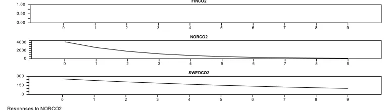
312
The graphic representation of these responses are represented in figures 3, 4 and 5 313
314
Responses to FINCO2
FINCO2
0 1 2 3 4 5 6 7 8 9
0 2000 4000
NORCO2
0 1 2 3 4 5 6 7 8 9
0 1000 2000
SWEDCO2
0 1 2 3 4 5 6 7 8 9
-2500 -500 1500
315
Figure 3. Representation of responses of shock in Finland emissions model
316
Responses to NORCO2
FINCO2
0 1 2 3 4 5 6 7 8 9
0.00 0.50 1.00
NORCO2
0 1 2 3 4 5 6 7 8 9
0 2000 4000
SWEDCO2
0 1 2 3 4 5 6 7 8 9
0 150 300
318
Figure 4. Representation of responses of shock in Norway emissions model
319
Responses to SWEDCO2
FINCO2
0 1 2 3 4 5 6 7 8 9
0.00 0.50 1.00
NORCO2
0 1 2 3 4 5 6 7 8 9
0.00 0.50 1.00
SWEDCO2
0 1 2 3 4 5 6 7 8 9
0 1500 3000
320
Figure 5. Representation of responses of shock in Sweden emissions model
321 322
These figures are in agreement with the three estimated models. 323
324
The forecast error variance decomposition
325 326
The point estimate of the impulse response function cannot reveal the whole consequences of 327
the unitary schock induced. As a help to evaluate more exactly this effect, we have the 328
forecast error variance decomposition. Now it is posible to assign the fraction of variance 329
error due to each of the variables: tables 6, 7, and 8. 330
331
In our case, with software RATS, we get: 332
333
Decomposition of Variance for Series FINCO2
334
Step Std Error FINCO2 NORCO2 SWEDCO2
335
1 4528.60958 100.000 0.000 0.000
336
2 5961.95795 100.000 0.000 0.000
337
3 6824.20457 100.000 0.000 0.000
338
4 7392.77638 100.000 0.000 0.000
339
5 7783.30602 100.000 0.000 0.000
340
6 8057.62382 100.000 0.000 0.000
341
7 8252.96153 100.000 0.000 0.000
342
8 8393.29461 100.000 0.000 0.000
343
9 8494.71357 100.000 0.000 0.000
10 8568.31098 100.000 0.000 0.000
345 346
Table 6. Error Variance decomposition for Finland emissions 347
348
Decomposition of Variance for Series NORCO2
349
Step Std Error FINCO2 NORCO2 SWEDCO2
350
1 4213.17694 1.023 98.977 0.000
351
2 5049.92138 1.023 98.977 0.000
352
3 5545.46136 7.029 92.971 0.000
353
4 5995.67688 16.398 83.602 0.000
354
5 6419.84339 25.531 74.469 0.000
355
6 6797.28532 32.968 67.032 0.000
356
7 7115.56081 38.590 61.410 0.000
357
8 7373.71297 42.717 57.283 0.000
358
9 7577.51608 45.716 54.284 0.000
359
10 7735.39086 47.893 52.107 0.000
360 361
Table 7. Error variance decomposition for Norway emissions 362
363
Decomposition of Variance for Series SWEDCO2
364
Step Std Error FINCO2 NORCO2 SWEDCO2
365
1 4013.45826 14.879 0.414 84.707
366
2 5402.49414 14.879 0.414 84.707
367
3 6199.38159 11.835 0.429 87.736
368
4 6771.28803 10.090 0.437 89.472
369
5 7246.87623 10.156 0.437 89.407
370
6 7677.85332 11.750 0.429 87.821
371
7 8083.39659 14.369 0.417 85.214
372
8 8468.41917 17.530 0.401 82.069
373
9 8832.16596 20.862 0.385 78.753
374
10 9172.28683 24.122 0.369 75.509
375 376
Table 8. Error variance decomposition for Sweden emissions 377
378
In the first column of these tables are printed the estimated standard errors of the predictions, 379
here 10 steps ahead. Each column shows the percentage of error due to each of the variables; 380
as a consequence the total of each row is 100. Once again, these tables are in agreement with 381
the three estimated models. 382
383
Forseeing the future
384 385
Once we get a validated model, we could attemp to forseen the future. From our simplified 386
The results are in table 9. 388
389
ENTRY FORECASTS(1) FORECASTS(2) FORECASTS(3) STDERRS(1) STDERRS(2) STDERRS(3)
390
2015:01 48081.8313 43906.7905 45265.4167 4528.6095 4213.1769 4013.4582
391
2016:01 48750.7476 41469.7532 46913.1434 5961.9579 5049.9213 5402.4941
392
2017:01 49323.5202 40065.1047 48259.2924 6824.2045 5545.4613 6199.3815
393
2018:01 49813.9680 39313.0813 49353.6138 7392.7763 5995.6768 6771.2880
394
2019:01 50233.9235 38966.9882 50238.0735 7783.3060 6419.8433 7246.8762
395
2020:01 50593.5185 38867.4508 50948.0349 8057.6238 6797.2853 7677.8533
396 397
Table 9. Forecasts of emissions for 2015 to 2020, and their standard errors 398
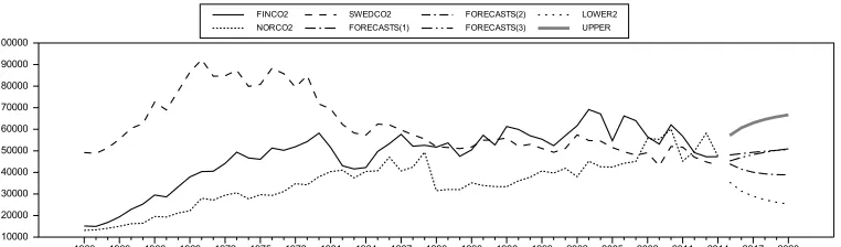
399
These results are represented in figure 2 400
401
FINCO2 NORCO2
SWEDCO2 FORECASTS(1)
FORECASTS(2) FORECASTS(3)
LOWER2 UPPER
1960 1963 1966 1969 1972 1975 1978 1981 1984 1987 1990 1993 1996 1999 2002 2005 2008 2011 2014 2017 2020 10000
20000 30000 40000 50000 60000 70000 80000 90000 100000
402
Figure 2. CO2 emissions 1960-2014 and their forecasts 2015-2010 with 95% confidence 403
bands 404
405
The picture shows that the Norvegian series is falling down, while the other two series show 406
a light rising path. 407
408
Results
409 410
Our VAR(2) model has established a classification among our series of CO2 emissions, with 411
the Finnish case been independent of the other two as well as affecting the CO2 emissions in 412
Norway and Sweden. Apart from the data series alone, the strong economy of Norway shows 413
a decreasing evolution in the inmediate near future. 414
415 416 417
Bibliography
418 419
Brown, L. R., The Great Transition, Shifting from Fossil Fuels to Solar and Wind Energy. 420
2015. New York. W. W. Norton. ISBN 978-0-393-35055-5. 421
Cryer, J. D. and Chang, K-S, Time Series Analysis with Applications in R, 2nd. ed. 2008. 423
New York. Springer Verlag. ISBN 978-0-387-75958-6. 424
425
Doan, Th., RATS v.9.2, 2017. Evanston, Illinois. Estima. 426
427
Doan, Th., RATS Handbook for Vector Autoregessions, 2nd. ed.. 2015. Evanston,Illinois. 428
Estima. 429
430
Hamilton, J. D., Time Series Analysis. 1994. Princeton. Princeton University Press. ISBN 431
978-0-691-04289-6. 432
433
Martin, V., Hurn, S. and Harris, D. Econometric Modelling with Time Series, Specification,
434
Estimation and Testing. 2013. Cambridge. Cambridge University Press. ISBN
435
978-0-521-13981-6. 436
437
Granger, C. W. J., Investigating causal relationships by econometric models and 438
cross-spectral methods. 1969. Econometrica, 37,424-438. 439
440
Granger, C. W. J. and Newbold, P. 1986. Forecasting Economic Time Series, 2nd. ed. 441
Orlando. Academic Press. ISBN 0-12-295183-2. 442
443
Lütkepohl, H. 2006. New Introduction to Multiple Time Series Analysis. Berlin Heidelberg 444
New York. Springer- Verlag. ISBN 978-3-540-26239-8. 445
446
R, R CORE TEAM (2017). R: A language and environment for statistical 447
computing. R Foundation for Statistical Computing, Vienna, Austria. 448
URL https://www.R-project.org/. 449
450
Shumway, R. H. and Stoffer, D. S. 2006. Time Series Analysis and Its Applications With R
451
Examples, 2nd ed. New York. Springer. ISBN 978-0-387-29317-5.
452 453
Tsay, R. S. 2010. Analysis of Financial Time Series, 3rd.ed. Hoboken. J. Wiley. ISBN 454
978-0-470-41435-4 455
456
Tsay, R. S. 2014. Multivariate Time Series Analysis with R and Financial Applications. 457
Hoboken. J. Wiley. ISBN 978-1-118-61790-8. 458
459
Tsay, R. S., MTS: All-Purpose Toolkit for Analyzing Multivariate Time Series (MTS) and 460
Estimating Multivariate Volatility Models, R pakage, version 033, 29-August-2016. 461
462
Woodward, W. A., Gray, H. L. and Elliot, A. C. Applied Time Series Analysis with R, 2nd. 463
ed. 2017. Boca Raton. CRC Press. ISBN 978-1-4987-3422-6. 464
Zivot, E. and Wang, J. 2006. Modeling Financial Time Series with S-PLUS, 2nd.ed. New 466
York. Springer. ISBN 978-0-387-27965-2. 467