Performance Analysis On Biplane Structure At Different Mach Numbers

Performance Analysis On Biplane Structure At

Different Mach Numbers

Nitin Kukreja, Sanjeev Kumar Gupta, Manish Kumar Rawat

Abstract: This paper summarize the optimized aerodynamic shape of the biplane geometry to get a significant reduction in wave drag, a significant viscous model to study aerodynamic shape of biplane is also found. Extensive results of numerical analysis shows that the optimized aerodynamic shape of the biplane geometry helps in finding a significant reduction in wave drag. The Spalart–Allmaras model is used as the viscous model in calculating the biplane structure. A broad study has been conducted on various grid sizes and the meshed geometries. Results show that the optimized model has certainly reduces the wave drag and the effect of flow-hysteresis. Through large number of test cases it has been also that the shockwave formation is diminished to a favorable limit.

Index Terms: Spalart–Allmaras; optimization; biplane; shockwave.

——————————  ——————————

1.

INTRODUCTION

Through the ages of transportation there are drastic developments in the field of aircraft efficiency and performance [1]. Air transport is known as the fastest means of transportation and optimization is always been the area of focus since its birth [1]. The occurrence of sonic booms limits the speed of the aircraft and the shockwaves generated at supersonic speeds results in unstable operation [2]. This study aims to realize a low-drag wing design that can improve the aerodynamic performance of the aircraft and is based on Busemann biplane concept. Computational Fluid Analysis of the flow suggests that the distribution of total lift into two separate wings can reduce the wave drag which is proportional to the square of the lift produced [2].

Fig. 1: Biplane of zero drag and noise [1]

This concept optimizes the design and increase the aerodynamic performance of the existing system [3]. A biplane is a two wing fixed one above the other. The main advantage of this geometry is that it reduces the drag in comparison to the normal wing to provide a high lift [4]. Bussemann biplane is an example of wave-drag reduction methods between two wings [5]. Bussemann biplane model inspired the creation of many models with other multiple elements leading to wave interactions in favorable condition and the reduction in wave drag [6]. Choked flow is formed when fluid flow through a restricted area whose rates reach maximum when the velocity reaches sonic at some point along the flow path [7]. Bussemann Biplane is renowned for utilizing favorable shockwaves collaboration to accomplish the nearly shockwave free supersonic flight at a particular Mach number [9]. The drag because of thickness can be significantly lessened by presenting the biplane setup.

Shape of Bussemann biplane

Fig. 2: Busemann biplane [1]

The biplane model can likewise essentially lessen the wave drag because of the airfoil thickness. Inside a supersonic meager close estimation, Busemann demonstrated that the wave drag of a zero-lifter Diamond can totally be eliminated by just parting the two components and those components are parallel to each other.

————————————————

 Nitin Kukreja, is currently working as an Assistant Professor – GLA

University, Mathura, PH-7409186806. E-mail:

[email protected].

 Sanjeev Kr Gupta, is currently working as an Assistant Professor – GLA University, Mathura, PH-9568188288. E-mail:

[email protected]

 Manish Kr Rawat, is currently working as an Assistant Professor – GLA University, Mathura, PH-8077270843. E-mail:

Fig. 3: Description of cancellation of waves [1] The solid stun wave produced at the main edge will precisely propagates to the inward corner and it will be crossed out by the development wave by then. At the outline condition, hypothetically the stun waves can be totally dropped out with the goal that zero wave drag occurs.

2

GEOMETRY

SETUP

2.1 Governing Equations

The theory that we have used to find out the lift and drag on mentioned airfoil is shock-expansion. A thin airfoil with small angle of attack was used. We have calculated lift an drag via through simple analytical expressions mentioned as in equation 1. The lift and drag coefficients as CL & Cd are

calculated through below mentioned formulas:

(1)

D/QC

=

C

L/QC,

=

C

Where, Q represents the dynamic pressure while C is the chord, L and d are the lift and wave drag of the airfoil, respectively. Also, The Euler equations for compressible inviscid flows can be written in an integral form

Fig. 4: Outline geometry of Busemann biplane X momentum:

(2)

(grad(u))

(

div

+

x

p/

-=

div(uV)

+

t)

u)/(

(











(3)

(grad(v))

(

div

+

x

p/

-=

div(vV)

+

t)

v)/(

(











2.2 Geometry Specification

The geometry model consists of two biplanes- triangular in shape placed one above the other. The distance between these two is 0.5 m and the length of each biplane is 4m, the distance between the two tips of the plane is 0.4 m.

2.3 Modeling of geometry

The geometry model is drawn using Gambit software. Using the coordinate system and the distance between two planes is 0.5m.

2.4 Boundary Layer

At some separation back from the main edge, the smooth laminar stream separates and moves in a turbulent stream. Boundary layer is created for accurate result on the boundary of the biplane. The first row is given as 1e-05 and 20 rows are given. The row density is very low at first so that there will be no clashing of grid after the grid generation. The boundary layer is created on all sliders, that is on three sides of biplane. The boundary layer is for knowing the exact position of result neat the wall.

Fig. 5: Boundary layer on the edges of biplane structure

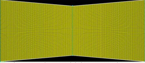
2.5 Grid Generation

The grid is generated in structured format. More dense mesh is created near the structure and low dense is created on the other parts of the structure. A rectangular type of grid is generated to know the external analysis of the structure. 200 vertical and horizontal nodes are given in between the two biplanes for dense mesh.

Fig. 7: More dense mesh in between two planes The figure shows the meshing for biplane model. We can see that mesh is denser near the walls and less dense at the outer surface. A closer look of it can be seen in the figure 8. We can observe from the above figure 8 that there is more dense mesh between two biplanes. This is because to get more accurate shocks.

2.6 Examination of the mesh

To make sure that the mesh is good in quality, examining the mesh is done. The result is that worst element is 0.154839.There are 400000 cells in the geometry after meshing.

Fig. 8: showing the quality of Mesh

3 SOLUTION

METHODOLOGY

3.1 Ansys Fluent Analysis

As demons The mesh file has been imported into the Ansys Fluent which consists of 400000 cells.

Fig. 9: Imported Mesh in fluent

3.2 Solution Methodology

Spalart-allmaras model is used as the viscous model in calculating the biplane structure. Here we have to use a turbulent model instead of laminar model. The Spalart-allmaras model is one equation model in turbulent viscosity type. This equation can solve the transport equations in

viscous types.

TABLE2

BOUNDARY CONDITIONS

S.No. Properties Value

1 Pressure type Far field

2 Gauge pressure 101325

3 Mach Number 1.7

4 Turbulent Viscosity ratio 2

5 Inlet temperature 300 K

6 Operating Pressure 0

7 Biplane Structure Wall

8 Wall motion Stationary wall

9 Shear condition No Slip

10 Heat flux across body 0

TABLE3

REFERENCE VALUES

S.No Properties Value

1 Area 1 m2

2 Density 1.1766 Kg/m3

3 Length 1 m

4 Velocity 590.0491 m/s

5 Ratio of specific heat 1.4

TABLE4

CONTROL PARAMETER

S.No. Properties Value

1 Formulation IMPLICIT

2 Flux type Roe-FDS

3 Spatial Discretization Gradient

Least Square cell based

4 Flow Second order upwind

5 Modified turbulent viscosity Second order upwind

6 Solution Control  Courant number  Solution initialization  Computation from  Reference frame

0.5 Standard

Inlet Absolute

TABLE1 GENERAL PROPERTIES

S.No Properties Values

1 Solver Density Based

2 Velocity formulation Absolute

3 Flow type Steady

4 Geometry Planar

5 Model Spalart–Allmaras

6 Density Ideal gas

7 Specific heat 1006.43 J/Kg-K

7 Monitors

 Continuity equation  Coefficient of drag  Coefficient of lift

10-6 Wall Wall

8 Run Calculation

 Number of iterations  Reporting interval  Profile update

104 1 1

4

RESULTS

After analyzing in fluent, the coefficient of drag and lift are obtained. We can observe from the results that there is formation of shocks between the two planes, from the validation of reference papers when compared to diamond air foil, the drag is around 0.0291. Whereas in Bussemann biplane analysis, it is clearly showing that the drag is very less than that of diamond airfoil which is 0.0088973969. The below figures shows the analysis of Bussemann biplane structures at Mach 1.7 has less drag coefficient.

Fig. 10: contours of Velocity at Mach number 3.0

Fig. 11: contours of Temperature at Mach 3.0

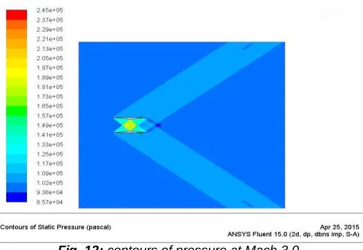
Fig. 12: contours of pressure at Mach 3.0

We can see that at Mach number of 1.7, the minimum pressure formed is 8.57×104and the maximum pressure formed is 2.45×104.

4.1 Pressure contour at different Mach Number

Fig. 13: Pressure contour at Mach 0.5

Fig. 15: Pressure contour at Mach 1.8

Fig. 16: Pressure contour at Mach 2.8

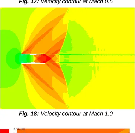
4.2 Velocity contours at different Mach numbers

Fig. 17: Velocity contour at Mach 0.5

Fig. 18: Velocity contour at Mach 1.0

Fig. 19: Velocity contour at Mach 2.0

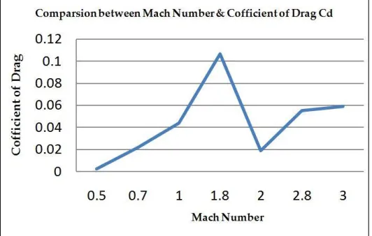
Fig 20: Depicts 3-Dimensional comparison between Coefficient of Drag on X-Axis for Bussemann Biplane & Mach

Fig 21: Depicts 2-Dimensional comparison between Coefficient of Drag on X-Axis for Bussemann Biplane & Mach

number on Y-axis

4 CONCLUSION

The classic 2D Bussemann biplane structures were modeled and the results were analyzed in fluent. We can deduce that there is reduction in drag in comparison with the other structures. 2-dimensional computational fluid dynamics results show that the used airfoil structure i.e. Busemann biplane airfoil produces very low wave drag. The reason of low wave drag is the presence of perfect shock wave cancellation. Through extensive literature studies and numerical findings, it has been also observed that the Busemann Biplane airfoil performance is poor for off-design conditions. A large set of case and data files based on inviscid compressible flow (Euler) explained the problem that how to overcome the choked-flow and flow hysteresis problems of the Busemann biplane under off-design conditions. Multiple design point strategy is used to obtain an optimized supersonic airfoil.

ACKNOWLEDGMENT

The authors wish to thank GLA University, Mathura for providing space for CFD Lab and for providing all kind of computational faclities.

REFERENCES

[1] Maruyama, D., Matsuzawa, T., Kusunose, K., Matsushima, K., and Nakahashi, K., ―Consideration at Off-design Conditions of Supersonic Flows Around Biplane Airfoils,‖ 45th AIAA Aerospace Sciences Meeting and Exhibit, AIAA Paper 2007-687, Jan. 2007.

[2] Yamashita, H., Yonezawa, M., Obayashi, S., and Kusunose, K., ―A Study of Busemann-Type Biplane for Avoiding Choked Flow,‖ 45th AIAA Aerospace Sciences Meeting and Exhibit, AIAA Paper 2007-688 Jan. 2007.

[3] Kuratani, N., Ogawa, T., Yamashita, H., Yonezawa, M., and Obayashi, S., ―Experimental and Computational Fluid Dynamics around Supersonic Biplane for Sonic-Boom Reduction,‖ 13th AIAA/CEAS Aeroacoustics Conference (28th AIAA Aeroacoustics Conference) AIAA Paper 2007-3674, 2007. [4] Kashitani, M., Yamaguchi, Y., Kai, Y., and Hirata, K., ―Preliminary

Study on Lift Coefficient of Biplane Airfoil in Smoke Wind Tunnel,‖ 46th AIAA Aerospace Sciences Meeting and Exhibit, AIAA Paper 2008–349, Jan. 2008.

[5] Maruyama, D., Matsushima, K., Kusunose, K., and Nakahashi,