Comparative Study of different methods used for GPS GDOP Approximation

Available online: https://edupediapublications.org/journals/index.php/IJR/ P a g e | 3168

Comparative Study of different methods used for

GPS GDOP Approximation

Madhu Ramarakula

1

, Gowthami Pagoti

2

1,2

Department of Electronics and communication engineering

University college of Engineering Kakinada

Kakinada- 533003,Andhra Pradesh, India

Email :

1

[email protected];

2

[email protected]

Abstract

The global positioning system(GPS), is a satellite based navigation system. Which is used in many applications such as communications, navigation, military, earth observation ,civil, and commercial user. So for correct position measurement, need to select best subset of satellites out of all combinations, which are used for finding user position. For this, the factor which helps in finding best subset of satellites from all the combinations is geometric dilution of precision(GDOP). It is a dimension less factor, which indicates the quality of the solution. the low GDOP value indicates the accurate solution. There are different methods for GDOP approximation, they are matrix inversion, closed loop algorithm, artificial neural networks. This paper compares GDOP approximation using these methods. The simulation results show that artificial neural networks have better accuracy than other methods.

Keywords

GPS, GDOP, Matrix inversion, closed loop algorithm, artificial neural networks

1.

Introduction

Now a days satellites plays an important role in day to day applications, such as communications, military, navigation, earth observation each. For navigation purpose global positioning system(GPS)[1] is used. It will send timing signals to GPS receiver, which is on the earth. The receiver calculate the distance between the satellite and receiver by using the timing signals and by using these distances the receiver will calculate its position.

1.1

GPS Structure

The GPS mainly consists of three segments. Those are space segment, control segment, user segment[2].

1.1.1 Space segment

The space segment consists of group of GPS satellites. Minimum 24 satellites distributed in six orbits are present in space segment and each will rotate with an inclination of ₅₅0 _{to cover the polar}

regions. At any time 5 to 8 satellites are visible from earth and minimum 4 satellites are required to determine the position of the user. The main function of space segment is to send and receive radio-navigation signals and also it will store and retransmit, navigation messages sent by control segment. By using this signal data the position of the user can be determined.

The satellite consists of solar panels, antennas, atomic clocks and radio transmitters. Each satellite have array of solar panels and these panels will produce energy by using sun light, these will provide this energy to satellites for their functioning. The satellite will rotate to point their solar panels towards the sun. The antenna present on satellite will send the signals generated by the radio transmitter in L-band to the GPS receivers. The radio transmitter present in satellite will generate the signals. These signals are ranging signals and navigation messages. The ranging signals are used for measurement of satellite distance from user. And usually this GPS satellites consists of two ranging codes, these are coarse/acquisition code(C/A code)and precision code(P code). C/A code is broadcasted by all the satellites but P code is used for military applications only.

The navigation message consists of ephemeris data i.e. used for calculating position of each satellite in the orbit and also almanac data, which has information about the time. For this signals transmission binary phase shift keying(BPSK) is used atomic clocks. These clocks are accurate in a billionth of a second. The inaccuracy of 1/100th of a second leads to a measurement error of 1860 miles o GPS receiver. By using these signals sent by the satellites the GPS receiver will calculate the user position by using trilateration.

1.1.2 Control segment

Available online: https://edupediapublications.org/journals/index.php/IJR/ P a g e | 3169 station(MCS), monitor stations, ground antenna. The

MCS plays an important role in all the control segment operations. The GPS satellites are tracked by the monitor stations by using pseudo range measurement and also these will receive the navigation messages from satellites. This raw data from all the monitor stations are send to the MCS through satellite communication system on ground. The MCS will process the all the data received from all the monitor stations for the satellite navigation payload control. And through this process the MCS will give satellite clock corrections and also almanac, ephemeris data of each satellite. And this updated data will be send back to the satellites through ground uplink antenna on S-band. Further satellites will send the required data to the GSP satellites through radio signals. And also MCS will monitor the satellite position at any instant of time, functioning of each satellite, variation in the navigation data and also the health of the satellite subsystem.

1.1.3 User segment

The user segment consists of GPS receiver. It will process the data i.e. ranging signals and navigation message to determine the user position and time by applying trilateration. And minimum four satellites are required for the computation of the position(X,Y,Z) and time. GPS receivers are mainly used for navigation, positioning and military.

There are so many factors which will cause the error in the data received by the user[3][4], they are propagation delay, receiver clock offset, satellite position geometry, satellite clock offset etc. The main factor which will cause the error is position calculation is satellite position geometry. At any time there are minimum 4 satellites are required to calculate the user position, if the selection of these satellites is not proper it leads to position error. So for accurate position calculation it is important to select best subset of satellites among all the combinations. This selection of subset of satellites is done by measuring the dimension less factor geometric dilution of precision(GDOP)[5][6]. It will show the quality of the solution i.e. it will give how much measured error effects the position solution error. The subset of satellites with less GDOP value gives better accuracy.

For his GDOP calculation different methods[7]-[9] are using such as matrix inversion, closed loop algorithm, and artificial neural networks. Among all these methods the better approach for getting best subset of satellites is to use matrix inversion for all the combinations and select the subset, which have the minimum GDOP value. But it is a time consuming process to calculate the GDOP value for all the combinations and also it will take around 160 floating point operations for each GDOP value

calculation. Another method used is closed loop algorithm which is similar to matrix inversion. But in this no need to calculate matrix inversion and also it perform 146 floating point operations. Another method used for selection of best subset of satellites is artificial neural networks. In this method no need to calculate big mathematical operations so it will decrease the computational burden and also improve the performance.

The distance between user and the satellite is

i

ˆ it is a pseudo range rather than range because accuracy errors effect the original range.

d i i ct

ˆ

(1)

Here

i

 is pseudo range and

t

_dis the receiver clock offset[10] and c is the speed of the light.

The pseudo-ranges can approximated by Taylor series expansion. Therefore, we obtain:

d i u i u i u

i  a a  b b  c c ct

 _{( )}2 _{( )}2 _{( )}2

(2) Here a_i,

i

b,ci are ith satellite position

coordinates, and c is the speed of the light, and (a_u,b_u,cu) are the user geometric coordinates.

d u i u i u i i i

i   h a h b h c ct 

 ˆ _{1 2 3}

(3) ; ˆ 1 i i n i s a a h  

i i n i s b b h  

ˆ 2 i i n i s c c h₃ ˆ 

(4)

Here

2 2

2 ₍ˆ _{) (ˆ )}

) ˆ

( _{n i n i n i}

i a a b b c c

s      

(5)                                                              d u u u n n n n t c c b a h h h h h h h h h 1 . . . . . . . . . . . . 1 1 . . . 3 2 1 23 22 21 13 12 11 2 1 (6) The general representation of the above matrix is

i





=R×a (7)

Here              1 1 1 1 43 42 41 33 32 31 23 22 21 13 12 11 h h h h h h h h h h h h

R (8)

Where R is a 4×4 direction cosine matrix „a‟ represents the user position, then the above equation can be written as

a=_R1 i 

 ₍₉₎ If the number of satellites are more than 4 that represents the system of equation is over determined. So, linear least squares approximation will be the solution to

a=_(RT_R)1_RT

i 

 ₍₁₀₎

Available online: https://edupediapublications.org/journals/index.php/IJR/ P a g e | 3170

2.Geometric dilution of precision

For the user position calculation minimum 4 satellites are required. But it is important to select the correct geometry of the satellites from which the signals are received. The calculated receiver position vary with selection of subset of satellites. So need to be careful while selecting the subset of satellites for the position measurement. The one factor used for

the selection of subset of satellites is

GDOP(geometric dilution of precision).It will basically measures satellite geometry i.e. it will tells the uncertainty in the satellite geometry. The low GDOP value leads to better accuracy.

The satellites should be arranged in orbit to minimize the chances of GDOP become large. If the satellite view from receiver is not clear i.e. by buildings the GDOP value may not be ideal. So for the accurate geometric position the receiver should have a clear view of the sky.

From equation (11) GDOP is consider as

) det(

)] ( [ )

( 1

N N adj trace N

trace

GDOP  

(12) From above equation GDOP value indicates the contributions of measurement error on position solution error for the particular subset of satellites. The higher GDOP value shows poor satellite geometry.

Table 1.GDOP ratings

GDOP value Ratings

1 Ideal

2-4 Excellent

4-6 Good

6-8 Moderate

8-20 Fair

20-50 Poor

3.

Closed loop algorithm

Hare N=RTR _{is the 4 × 4 matrix having four Eigen}

values

i

k(i = 1, 2, 3, 4). As we know trace of the

matrix is the summation of the eigen values so eigen

value of 1

)

(RTR  is 1 i

k

by rewriting the equation (12)[3]

1 4 1 3 1 2 1 1 1 )

(         

 trace N k k k k

GDOP

(13) In the above equation for calculating GDOP value it needs to be perform the matrix inversion but the closed loop algorithm[11] easy the calculation by using the following equations, and these will decrease the number of operations.

p

1



k

1



k

2



k

3



k

4



trace

(

N

)

₍₁₄₎

)

(

2

2 4 2 3 2 2 2 1

2

k

k

k

k

trace

N

p











(15)

) ( 3 3

4 3 3 3 2 3 1

3 k k k k trace N

p     

(16)

) det(

4 3 2 1

4 kk k k N

p   ₍₁₇₎

Hare N is symmetric matrix so all the above equations are valid. After finding the common denominator, the above equation for GDOP changes to the value of GDOP is given as follows(4):

4

3 2 1 3

1 3

5 . 15 5 . 0

p

p p p p

GDOP  

(18) This equation gives us a 4 to 1 mapping of inputs and outputs.

This method will decrease the computational burden for calculation of matrix inversion. And also decrease the floating point operations required for GDOP calculation.

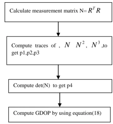
The below figure shows the GDOP approximation using closed loop algorithm.

Fig1. GDOP computaion using closed loop algorithm

4.

Neural network based approximation

Human neuron system has billions of neuron cells, which will process the information and each cell works as a processor. Each neuron has dendrites, soma, axon, synapses. The dendrites in neuron receive he activation signal from the other neurons. Soma in neuron will process the activation signals received from dendrites and produce the output activation signals. The axon will send the activation signals from one neuron to another neuron. The junctions in neurons i.e. synapses allow the transmission of signal between dendrites and axons. Artificial neural networks(ANN) are designed based on the human neural system. In this one neuron is connected to another neuron via synapses through the weights. Weights acts as a connection link between the two neurons. Here each input is multiplied with respective weights and processing unit will sum up all the inputs and apply the activation function to the resultant value and the activation function will perform the mathematical

Calculate measurement matrix N=

R

T

R

Compute traces of ,

N

N

2,

N

3,to get p1,p2,p3

Compute det(N) to get p4

Available online: https://edupediapublications.org/journals/index.php/IJR/ P a g e | 3171 operations and produce signal output and this output

will send to other neurons. Basically ANN is does not have any particular mathematical model, so these can be used o solve wide variety problems. So it can be used for GDOP approximation[12]-[14]. It is basically a three layer structure. Every layer is connected to another layer via weights. And after every iteration these weights are updated according to the error, which is the difference between network actual output and the desired out put. The learning rule in ANN tells that how these weights should be updated to decrease the error value. The problem solving using ANN will be done in two phases i.e. approximation and classification. In approximation it will calculate values for the available solutions, where as in classifier it will select the one of the optimal solution.

The single layer feed forward network has only single layer of weights. The input layer directly connects to output layer via weights. The connection of input to output is only in one direction there is no feedback connection so it is called as feed forward network. If the sum of product of input and weights is crosses a threshold value the output will return a 1 value otherwise it will return a 0 value.

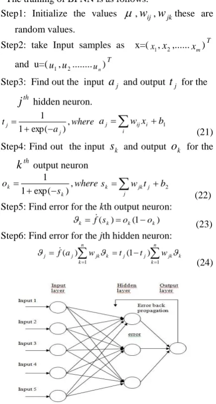
The multi layer feed forward network has three layers. Those are input layer, output layer, and hidden layer. Each layer connects to another layer through weights. The hidden layer will perform the intermediate computation before sending the input value to the output. The recurrent network has atleast one feedback path the output from the output layer will be sent back to the input layer through the feedback path i.e. the output of a neuron will feedback itself as input.

4.1 The Back-propagation Neural Network

(BPNN)

The most used learning algorithm in all the neural networks is back propagation neural networks[15]. It is basically a multi layer feed forward network. And it has input, output, hidden layers The output input layer is used to activate the hidden layer, and also output of hidden layer is used to activate the output layer. Any mapping of input variables to output variables m_n _{can be done by using a three layer}

structure[16] (i.e. input layer, hidden layer, output layer)this is explained by the Kolmogorov's Theorem. The training for neural networks is done for minimizing the error, if a se of input samples are available it will update the weights to minimize the following squared error.







 n

k

k

k o

u E

1

2 ) ( 2 1

(19) Here n is the number of output variables

The nodes in neural networks transform the ne input by using activation function here it will use the sigmoid function as the activation function.

) exp( 1

1 )

(

t t

f

  

(20)

Net input to the particular layer can be obtained by the summation of the multiplication of the weights with the previous layer inputs. And also hidden and output nodes will use a bias value for computing the input to the particular layer. Here bias is a connection weight with a constant activation value from a special unit.

The training of BPNN is as follows:

Step1: Initialize the values



,

w

_ij,

w

_jkthese are

random values.

Step2: take Input samples as x=(x₁,x₂,...x_m)T

and u=(u₁,u₂..._un)T

Step3: Find out the input

a

_j and output

t

_j for the

th

j

hidden neuron.

where a

t

j

j ,

) exp( 1

1

 

 a w x b1

i i ij

j 





(21)

Step4: Find out the input

s

_k and output

o

_k for the

th

k

output neuron

where s

o

k

k ,

) exp( 1

1

 

 s w t b2

j j jk

k 





(22) Step5: Find error for the kth output neuron:

) 1 ( )

( k k k

k f s o o

 ₍₂₃₎

Step6: Find error for the jth hidden neuron:





 

   n

k

n

k k jk j j k jk j

j f a w t t w

1 1

) 1 ( )

(  

 

(24)

Fig 2. The topology of a three-layer back-propagation neural network.

Step7: calculate w_jk,w_ij:

j k

jk t

w 



,

i j

ij x

w 





Step8: update weights

w

_jk,

w

_ij:

w

_jk



w

_jk





w

_jk,

ij ij

ij

w

w

w







(25) Step9: calculate the error value

_





 n

k k k o u E

1 2 ) ( 2

1 (26)

Available online: https://edupediapublications.org/journals/index.php/IJR/ P a g e | 3172 Here

µ : learning rate,

i

x

: ith input neuron value ,

j

t

: jth hidden neuron output,

k

u

: kth output neuron‟s desired output,

k

o

: kth output neuron‟s actual output,

ij

w

:ith input neuron and the jth hidden neuron inter connection weight,

jk

w

: jth hidden neuron and the kth output Neuron inter connection weight.

5.Gdop approximation using BPNN

BPNN is basically a three layer structure. It is taken from Kolmogorov's Theorem where it states that any input output mapping m_n

can be represented by three layers. In this input variables are mapped with output variables.

Here mapping of inputs to the outputs is done by the four inputs to one output mapping

) ( 4

3 2 1

1 k k k k trace N

p      ₍₂₇₎

) ( 2 2

4 2 3 2 2 2 1

2 k k k k trace N

p      ₍₂₈₎

) ( 3 3

4 3 3 3 2 3 1

3 k k k k trace N

p      ₍₂₉₎

) det( 4 3 2 1

4 kk kk N

p   ₍₃₀₎

This network will perform a 41 _mapping

from k_i to GDOP, i.e. _{p GDOP}

i here we are using

a simple (4-3-1) structure

Input: (

x

₁,

x

₂,...

x

_m)T=

(

k

₁

,

k

₂

,

k

₃

,

k

₄

)

T

Output: y=GDOP

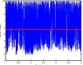
6.Results

The Simulation was conducted to compare the performance for the GDOP approximation for three methods. GDOP is calculated for every subset of 4 satellites. For comparing performance, all the three methods are experimented with around 30000 learning iterations. The learning rate is chosen as 0.5. The input variables, _{k i} and RTR_{, values were} normalized to range [0, 1] , and the output variable GDOP value, was normalized to 0.2. and the Results showed that, after 30000 learning iterations, the neural network method shows better GDOP accuracy than the matrix inversion and closed loop algorithm.

0.5 1 1.5 2 2.5 3

x 104 1

2 3 4 5 6 7 8 9 10

Total iterations

G

D

O

P

v

a

lu

e

Fig 3.GDOP approximation by matrix inversion

0.5 1 1.5 2 2.5 3

x 104 1

2 3 4 5 6 7 8

Total iterations

G

D

O

P

v

a

lu

e

Fig 4. GDOP approximation using Closed loop algorithm.

0.5 1 1.5 2 2.5 3

x 104 1.5

2 2.5 3 3.5 4 4.5 5 5.5 6

Total iterations

G

D

O

P

v

a

lu

e

Fig 5. GDOP approximation using back propagation neural networks

The below shows the average GDOP values for three methods

Table2. Average GDOP of three methods

Method Average GDOP

Matrix inversion 5.6690

Closed loop algorithm 5.0055 Back propagation neural networks 4.2060

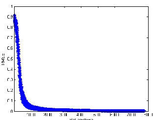
The root-mean-squared error (RMSE):

It is the error used for evaluating the approximation performance.

n o o RMSE

n

k

MI NN





  1

2 ) (

(31)

Available online: https://edupediapublications.org/journals/index.php/IJR/ P a g e | 3173 Figure 7 shows the graph between RMSE and

number of iterations.

Fig 6. graph between RMSE and number of iterations.

7.Conclusion

The GDOP value indicates the how well the GPS satellite geometry is organized. GPS positioning with a low GDOP value usually gains better

accuracy. GDOP approximation for Different

methods have been successfully conducted. The viewpoint of accuracy, all the three methods provide sufficiently good performance, but neural network method have a good accuracy compared to remaining two methods. But it has some drawback that it has a slow learning time. We conclude that, a neural network model is superior when compared to matrix inversion or closed loop algorithm while filtering the redundant GDOP from required GDOP.

8.Future scope

The neural network, even though approximates the data efficiently, has a slow learning rate and is predominantly a binary classifier. This can be improved further by using a linear classifier such as a Support Vector Machine or other kernel based regression techniques.

9.References

[1] A. EI-Rabbany, “Introduction to GPS: The Global Positioning System”. Boston, MA: Artech House, 2002.

[2] L.F.Wiederholt and E.D.Kaplan : GPS system segments: in understanding GPS: principles and applications. ed. by E.D.Kaplan,C.J.Hegarty(artech house, norwood 2006) pp.67-112

[3] V. Ashkenazi, “Coordinate systems: How to get your position very precise and completely wrong,” J. Navig., vol. 39, no. 2, pp. 269–278, May 1986. [4] T.-K. Yeh, C.-S.Wang, C.-W. Lee, and Y.-A. Liou,

“Construction and uncertainty evaluation of a calibration system for GPS receivers,” Metrologia, vol. 43, no. 5, pp. 451–460, Oct. 2006.

[5] J. Zhu, “Calculation of geometric dilution of precision,” IEEE Trans. Aerosp. Electron. Syst., vol. 28, no. 3, pp. 893–895, Jul. 1992.

[6] Teng, Yunlong, Jinling Wang, and Qi Huang. "Mathematical minimum of geometric dilution of precision (gdop) for dual-gnss constellations", advances in space research, 2016.

[7] M. R. Mosavi. "Efficient evolutionary algorithms for GPS satellites classification", arabian journal for science and engineering, 05/05/2012.

[8] M. R. Mosavi. "knowledge-based methods for optimum approximation of geometric dilution of precision", international journal of computational intelligence and applications, 2010.

[9] Pei-Yi Hao, , and Chao-Yi Wu. "GPS GDOP approximation using support vector regression algorithm with parametric insensitive model", 2012 international conference on machine learning and cybernetics, 2012.

[10] P. Misra and P. Enge, Global Positioning System: Signals, Measurements, and Performance, 2nd ed. Lincoln, MA: Ganga Jumana Press, 2006.

[11] S.-H. Doong, “A closed-form formula for GPS GDOP computation,” GPS Solutions, vol. 13, no. 3, pp. 183–190, Jul. 2009.

[12] D. Simon and H. El-Sherief, “Navigation satellite selection using neural networks,” Neurocomputing, vol. 7, no. 3, pp. 247–258, Apr. 1995.

[13] Azarbad, Milad, Hamed Azami, Saeid Sanei, and Ataollah Ebrahimzadeh. "New neural network-based approaches for GPS GDOP classification based on neuro-fuzzy inference system, radial basis function, and improved bee algorithm", applied soft computing, 2014.

[14]D. J. Jwo and C. C. Lai, “Neural network-based GPS GDOP approximation and classification,” GPS Solutions, vol. 11, no. 1, pp. 51–60, Jan. 2007. approximators,” Neural Networks, vol. 2

[15] D. J. Jwo and K. P. Chin, “Applying back-propagation neural networks to GDOP approximation,” J. Navig., vol. 55, no. 1, pp. 97–108, Jan. 2002.