An Iterative Threshold Algorithm Based on Log-sum Norm
Regularization for Magnetic Resonance Image Recovery
Lin Yu Wang, Ming Qi He*, Jian Hong Xiang, and Peng Fei Ye
Abstract—This paper considers the class of Iterative Shrinkage Threshold Algorithm (ISTA) to solve the linear inverse problem that occurs in magnetic resonance (MR) image recovery. The ISTA algorithm adheres to the principle of minimizing the L1 norm. This method can be considered as an extension of the classical gradient algorithm. However, it is known that the ISTA algorithm converges slowly, and the accuracy of the algorithm is not sufficient. In many MR image recovery problems, using non-convex log-sum norm minimization can often obtain better results than the l1-norm minimization. In this paper, we firstly transform the MR image recovery into a non-convex optimization problem with log-sum norm regularization and combine it with a faster global convergence method. Then a Log-sum generalized iterated shrinkage threshold algorithm (LISTA) for solving the MR image recovery problem is proposed. Finally, numerical experiments are conducted to show the superiority of our algorithm.
1. INTRODUCTION
MR image recovery plays a vital role in clinical diagnosis. However, at present, the quality of MR image recovery needs to be strengthened. Compressed sensing (CS) is a new sampling technique applied to MR imaging recovery. The CS first acquires a small amount of k-space data (also called Fourier coefficients) to shorten the image recovery time, then reconstructs the MR image from the undersampled data. Assuming the image is sparse, we can recover the image from a small number of Fourier coefficients. Therefore, we need to find an image that is sparse in the transform domain to fit the undersampled k-space data. We can transform the MR image by transforming domain (such as DCT, Fourier, wavelet), so that CS can be applied to MR image recovery. There have been some studies showing that the MR image restoration problem is a morbid inverse problem, so the commonly used image reconstruction method is to add regularization to the problem. MR image recovery based on compressed sensing mainly concerned with the problem of so-called sparseness constraint minimization, and image restoration is often achieved by sparse minimization. One difficulty with the sparse constraint minimization problem is the choice of minimized norm. In recent years, Daubechies et al. proposed iterative shrinkage thresholding algorithm (ISTA) [1] based on the L1 norm regularization problem and successfully applied it to MR image recovery. The ISTA idea is relatively simple. It only needs to determine the initial value of the algorithm, step size, and denoising operator, and achieve the convergence effect by the gradient descent. Then, under the framework of the ISTA algorithm, Beck and Teboulle proposed the Fast Iterative Shrinkage-Thresholding Algorithm [2] to improve the convergence speed of the algorithm. Based on ISTA algorithm, a two-step iterative shrinkage threshold algorithm is proposed in [3], which is also based on the idea of improving the algorithm speed. Inspired by the ISTA that solves the L1 regularization problem, Zuo et al. proposed a generalized iterative shrinkage thresholding algorithm (GISA) [4] to solve the Lp regularization problem. Compared with ISTA, GISA uses different methods
Received 3 November 2019, Accepted 2 January 2020, Scheduled 13 January 2020
* Corresponding author: Ming Qi He ([email protected]).
of contraction operator, while the iteration form is almost the same as ISTA. Then some scholars have made further improvement based on GISTA algorithm, and proposed FGISTA algorithm [5]. FGISTA algorithm improves the speed of GISTA algorithm, but the accuracy is decreased. Based on the p-norm, Chartrand and Yin proposed an Iterative Reweighted Least Squares (IRLS) algorithm [6]. Unlike gradient descent, the algorithm uses the least squares method to converge. Paper [7] proposes to apply
l1
2 norm to iterative threshold algorithm, which further extends the compressed sensing algorithm. Now, this kind of compressed sensing algorithm is widely used in various fields, such as image restoration [8– 10] and MRI imaging [11], because of its strong scalability.
There are still a lot of studies on the problem of minimizing the norm. Some scholars have suggested in the literature [12–14] that the log-sum norm can effectively approximate the L0 norm and prove that the log-sum norm can also be used as a regularization term.
2. RELATED WORK
Previous studies of MR image recovery have shown that using L0 norm minimization usually yields good results, and it is designed to address the following minimization problems:
min1
2||y−Ax||
2+λ||x||
0 (1)
where yis an n×1 vector, A a sensing matrix, x the the original signal (or image), and ||x||0 simply
counts the number of non-zero entries inx. Unfortunately, the L0 norm is a non-convex non-continuous function, which makes the corresponding solution problem very cumbersome.
Since the L1 norm is a convex hull of L0 norm and has the property of continuity, many researchers have shifted the study to the L1 norm. It has been proved that the L1 norm minimization is equivalent to the L0 norm minimization when A satisfies certain conditions [15, 16]. Unlike solving the L0 norm minimization, many algorithms seek the desirexby solving the following convex optimization problem:
min1
2||y−Ax||
2+λ||x||
1 (2)
In solving [2], the fast iterative shrinkage-thresholding algorithm (FISTA) which is based on the gradient descent method makes smarter choices in the iterative process to obtain the ideal solution. In ISTA algorithm, Donoho proposed a soft threshold operator [16], which is defined as:
T1(y;λ) =
0, |y| ≤λ
sgn(y)(|y| −λ) |y|> λ (3)
Based on the ISTA algorithm, FISTA improves the selection of the starting point and improves the convergence speed of ISTA algorithm. The difference between the two algorithms is the choice of the initial position.
To solve the L1 norm problem, the GISTA algorithm gives a model using the p-norm:
min1
2(y−Ax)
2+λxp (4)
Like the traditional iterative threshold method, GISTA algorithm needs to approximate the convergence image by gradient descent. However, GISTA needs to define its p value according to different noise intensities and different images in order to get better reconstruction effect.
In order to solve the problem in Eq. (1), some researchers have proposed the optimization problem of the log-sum norm, which is expressed as:
min1
2(y−Ax)
2+λlog(x+u) (5)
This paper mainly discusses the MR image recovery problem based on log-sum norm constraint. Based on the ISTA algorithm, a Log-sum generalized iterated shrinkage threshold algorithm (LISTA) for solving Equation (5) is presented.
So far, various algorithms have been proposed to minimize the norm in MR image recovery. The process of obtaining the sampled MR image can be expressed as:
y=Ax+η (6)
whereA is a sampling matrix or sensing matrix,x the original image, η the noise, andy the acquired compressed signal (or image). The MR image recovery problem is the process of recovering the ideal imagexfrom the compressed image y. Since the sampling matrixA is a highly ill-conditioned matrix, the problem is an ill-posed inverse problem, and a common method for solving ill-conditioned problems is to regularize it.
This paper mainly considers the MR image recovery problem based on log-sum norm regularization:
min1
2||y−Ax||2+
n
i=1
λlog(|xi|+ε) (7)
where 12||y −Ax||is often referred to as the data fitting term, and λlog(|xi|+ε) is the penalty term.
εacts as a regularization, balancing the value of the function f(x) when xis too small, and it usually takes from 0.01 to 0.001. LISTA algorithm adopts the idea of the ISTA algorithm based on the log-sum norm as the penalty term, and its core is to find a contraction operator similar to the iterative threshold class algorithm.
3. MAIN RESULTS
The core of the ISTA algorithm is the gradient descent method. The unconstrained optimization problem is as follows:
min
x {F(x) =f(x)} (8)
where f(x) is the formula 12||y−Ax||2. Assume that f(x) is continuously differentiable, if there is a
small enough value tk >0 such thatxk+1 =xk−t∇F(xk) , then:
F(xk)≥F(xk+1) (9)
Thexkvalue corresponding to the minimum value of the functionf(x) can be obtained by iterating through the following steps:
xk =xk−1−tk∇f(xk−1), x0 ∈Rn (10)
The ISTA algorithm assumes that f(x) satisfies the Lipschitz continuous condition, that is, the derivative of f(x) has a lower bound, and the minimum lower bound is called the Lipschitz constant
L(f). At this time, for any L >=L(f), there are:
f(x)≤f(y) +x−y,∇f(y)+L
2||x−y||
2 x,y∈Rn (11)
Based on Eq. (11), the function value can be approximated near pointxk:
ˆ
f(x, xk) =f(xk) +∇f(xk),x−xk+ L
2||x−xk||
2 (12)
Adopting this same basic gradient idea to the nonsmooth L1 regularized problem:
min
x {F(x) =f(x) +λ||x||1} (13)
After bringing the function into the penalty, the value of the function can be approximated by the point xk:
ˆ
f(x, xk) =f(xk) +∇f(xk),x−xk+L
2||x−xk||
2+λ||x||
In each iteration of gradient descent, the approximation function of pointxk−1takes the minimum
point as the starting point xk of the next iteration:
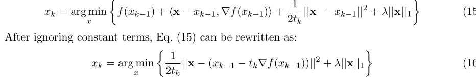
xk = arg min x
f(xk−1) +x−xk−1,∇f(xk−1)+
1
2tk||x −xk−1||
2+λ||x|| 1
(15)
After ignoring constant terms, Eq. (15) can be rewritten as:
xk= arg min x
1
2tk||x−(xk−1−tk∇f(xk−1))||
2+λ||x|| 1
(16)
Inspired by ISTA, we propose a generalized shrankage thresholding operator to solve the log-sum minimization problem in Eq. (5) by modifying the shrinkage rules. We convert the L1 norm regularization into a log-sum norm regularization problem and simplify it based on Eq. (16), which is expressed as:
xk = arg min x
1
2tk||x−(xk−1−tk∇f(xk−1))||
2+
n
i=1
λlog(|xi|+ε)
(17)
In order to facilitate the analysis of the change in the concavity, we turn the above formula into the simplest logsum norm minimization problem:
min 1
2tk(x−y)
2+λlog(x+ε) (18)
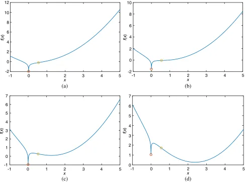
wheretkis the step size and is generally taken as 1. λis known as regularization strength, and its value range is generally (0, 1]. Ify>0, the solution to Eq. (18) should fall into the range of [0,y]. If y<0, the solution into the range of [y, 0]. Without loss of generality, in the paper we only consider the case
y>0, and we settk= 1 andλ= 0.3. In Fig. 1, we take four different values fory. It can be seen from Fig. 1 that there is a threshold τlog-sum. When y< τlog-sum, then 0 is the value of x corresponding to
the global minimum. When y> τlog-sum, the local minimum and zero values need to be compared.
For the non-convex problem, if the contraction rule of the ISTA algorithm is directly adopted, x
can generally only shrink to the local minimum rather than the global minimum. Therefore, we need to set a threshold τlog-sum to judge various situations. First, we need to determine if the function has a
local minimum.
We can analyze the convergence of the function by the first derivative and the second derivative of
f(x).
f(x) =x−y+t
kλx+1 ε
f(x) = 1−λt
k 1
(x+ε)2
(19)
We can get this inflection point by the second derivative of the functionf(x). The inflection point coordinates arexλ =√λtk−ε. We can see from Fig. 1 that whenx> xλ, the functionf(x) is concave; otherwise, it is convex. If the function has a local minimum, f(xλ) ≤0. Based on this, we can get a threshold by the following formula.
f(xλ) =xλ−y+tkλ 1
xλ = 0 (20)
We can get the threshold ofy:
τλtk =
λtk−ε+√λtλtk
k−ε (21)
However, it is easy to find through c in Fig. 1: even if the function f(x) has a local minimum, it needs to compare the size with f(0) to determine the global minimum. As shown in Fig. 1(d), wheny
-1 0 1 2 3 4 5
x
(a) (b)
(c) (d)
-1 0 1 2 3 4 5
x
-1 0 1 2 3 4 5
x
-1 0 1 2 3 4 5
x 12 10 8 6 4 2 0 -2 f ( x ) 10 8 6 4 2 0 -2 f ( x ) -1 0 1 2 3 4 5 6 7 f ( x ) 0 1 2 3 4 5 6 7 f ( x )
Figure 1. Plots of the functionf(x) in Eq. (18) with different values of y: (a)y= 0.5, (b)y= 1, (c)
y= 1.5, (d) y= 2.5.
the critical point is ˜x, an approximate estimate of ˜xcan be obtained by the formulaf(˜x) = f
x→0
(x) and
f(˜x) = 0:
˜
x−τx+tkλx˜+1ε = 0
f(˜x) = f
x→0
(x) (22)
However, the solution to this equation is a transcendental equation, and we can only get an approximate solution through matlab. Based on this, we can get an approximation of estimate
˜
x≈ √ε2+8tkλ−ε
2 . The regularization factor εis generally taken as [0.01, 0.001], so its quadratic square
can be ignored. Therefore, ˜x≈√2tkλ−ε/2. τx corresponding tox is taken as its threshold. Then the approximate estimate of the threshold ˜τx is:
˜
τx=2tkλ−ε 2 +
tkλ √
2tkλ+ε/2 (23)
Now we can draw conclusions. Whenyis greater thanτlog-sum, we can judge that functionf(x) has
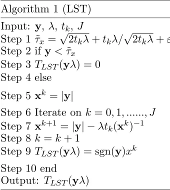
Table 1. The left is the log-sum contraction operator corresponding to the LISTA algorithm, which is LST. The right is the total LISTA algorithm step.
Algorithm 1 (LST) Algorithm 2 (LISTA)
Input: y,λ,tk, J Input: y,λ,tk,J, iter
Step 1 ˜τx =√2tkλ+tkλ/√2tkλ+ε Step 1 Initializex0 =y,z0 =x0
Step 2 if y<˜τx Step 2 fork= 1: iter
Step 3 TLST(yλ) = 0 Step 3y=zk−1−tkAT(Azk−1−y) Step 4 else Step 4xk =LST(y, λ, tk, J)
Step 5 xk=|y| Step 5lk= (1 +
1 + 4(lk−1)2)/2
Step 6 Iterate on k= 0,1, ..., J Step 6zk=xk+lk−l1k−1(xk−xk−1) Step 7 xk+1=|y| −λt
k(xk)−1 Step 7x=xiter
Step 8 k=k+ 1 Step 8 end
Step 9 TLST(yλ) = sgn(y)xk Output: x
Step 10 end Output: TLST(yλ)
minimum value. WhenJ is too small, the total number of iterations of LISTA algorithm will increase, resulting in the increase of the total time.
The above is the operator that selects the minimum value, and the body of the LISTA algorithm is similar to the ISTA algorithm. We introduce the above iterative contraction operator based on the ISTA algorithm and add the acceleration operator of the FISTA algorithm to the LISTA algorithm. The corresponding algorithm is shown in the right of Table 1.
4. NUMERICAL EXAMPLE
In this section, we will present numerical results to illustrate the efficiency of our proposed algorithm. We firstly compare the efficiencies of the LISTA algorithm in radial sampling matrix at different sampling rates. In the second subsection, we will compare FISTA, GISTA, LISTA, then we also select several state of the art methods for comparisons. In the last subsection, we will analyze the convergence of different algorithms under different iterations. The test MR images are mainly taken from the medical image library, shown in Fig. 2, and we add a Gaussian noise with a standard deviation of 1e-2 to the test.
4.1. Evaluation Criterion
In this subsection, we use SSIM, peak signal-noise ratio (PSNR), and running time to evaluate the quality of restoration, which are defined as:
MSE = ||x−xˆ||2/(M×N) (24)
PSNR = 10 lg(2552/MSE) (25)
SSIM(p, q) = (2μpμq+c1)(2σpq+c2) (μ2
p+μ2q+c1)(σp2+σ2q+c2)
(26)
where ˆx and xdenote the original and restored image respectively, andM and N represent the length and width of the picture. We also consider the running time of every algorithm. SSIM is a new indicator to measure the structural similarity between two images. In image restoration, the larger the SSIM value is, the better the image restoration quality is. μp is the mean of image p, and μq is the mean of image
q. c1 =k1L and c2 =k2L, in which k1 is 0.01, and k2 is 0.03. L is the dynamic range of pixel values.
σp and σp are the variance of image. σpq is the covariance between two images.
We conduct some experiments to illustrate the superiority of the LISTA algorithm in MR image recovery. In the selection of parameters, we uniformly set the step size tk to 0.5. The range of regularization parameters λ is generally (0, 1]. In past experiments, the selection of regularization parameters λ based on changes in noise intensity could yield better MR image recovery results, so we set the regularization parameterλto 1 under this low noise condition. For GISA algorithm, we choose
p= 0.8 (thepvalue is also chosen in the original paper.) for the comparison. For FISTA algorithm, the regularization strength is the same as LISTA algorithm, which is taken as 1. For fairness, according to other references, we can obtain satisfactory results by uniformly selecting J = 2 or 3, so we set J = 2. All experiments are operated under Windows 10 and MATLAB R2016a with the platform of Intel (R) Core (TM) i5-7th Gen [email protected] GHz 2.50 GHz.
Next, we will carry out our experiments from three aspects: 1) reconstruct the same MR image at different sample rates. 2) analyze the peak signal to noise ratio (PSNR) of different algorithms. 3) analyze the convergence of the algorithm under certain noise conditions.
4.2. Performance Evaluation of Different Sample Rates for MR Image Recovery under the Same Conditions
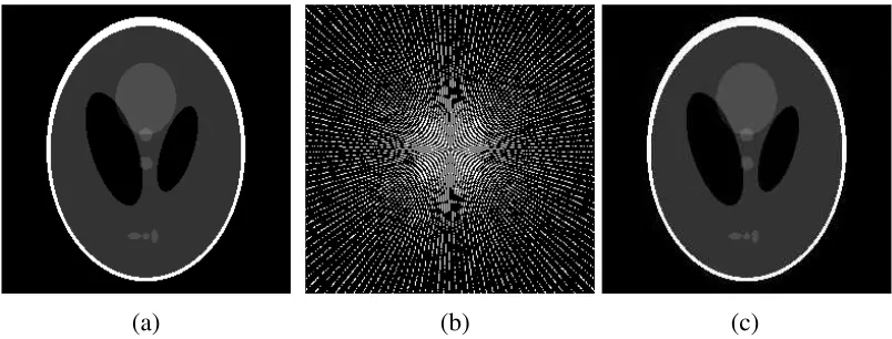
First, we display the original image of the MR image. The selected sampling matrix is a radial sampling matrix under the Fourier domain. In the experiment, the sampling rate of the matrix is 30%; the obtained reconstructed image PSNR is 38.44 dB; reconstruction time is 0.712 seconds. The result is shown in Fig. 3. From Fig. 3, we can find that under the 30% sampling matrix, our algorithm can reconstruct the MR image effectively.
(a) (b) (c)
Table 2. Comparison of PSNR and time after restoration of MR images of LISTA algorithm under different sampling matrices.
Sampling Rate PSNR (dB) SSIM (%) time (s)
20% 28.96 65.88 0.65
30% 38.44 95.54 0.71
40% 44.20 98.05 0.74
50% 47.58 98.90 0.75
From Table 2 we can see that when the sampling rate is greater than 30%, LISTA algorithm works well on reconstructing MR images, with PSNR greater than 38 dB and SSIM greater than 90%. As the sampling rate increases, the effect of reconstructing the MR image is better. It can be seen from Table 2 that an increase in the sampling rate will increase the time. However, this result verifies the superiority of compressed sensing compared to Nyquist sampling. The LISTA algorithm can reconstruct MR images with superior quality by reducing the sampling rate.
4.3. Performance Evaluation of Different Algorithms
In order to eliminate the influence of random factors on the algorithm results, we use the 30% sampling matrix to test different images. The parameter selection is the same as 4.1. We use GISTA, FISTA and LISTA algorithms to perform the recovery of PSNR of the MR image after testing 100 times. The experimental picture is shown in Fig. 4. The specific data are shown in Table 3. It can be seen from
(a) (b) (c)
(d) (e) (f)
Table 3. Comparison of effects of LISTA, GISTA and FISTA algorithms in MR image reconstruction.
image algorithm PSNR (dB) SSIM (%) time (s)
image 1
FISTA 27.08 0.861 0.648
GISTA 28.00 0.931 0.689
LISTA 28.94 0.941 0.734
image 2
FISTA 35.20 0.922 0.870
GISTA 36.06 0.932 0.880
LISTA 36.08 0.944 0.877
Table 3 that the algorithm effect of LISTA is good for different algorithms. These experiments show that the LISTA algorithm is more accurate than other algorithms under low noise conditions.
Combined with Table 3 and Fig. 4, FISTA is less accurate than other algorithms but with less time, and GISTA algorithm is somewhere in between. The accuracy of the proposed LISTA algorithm has been improved, both in SSIM and PSNR. We can see that LISTA algorithm has reached the standard of the iterative threshold class algorithm and even surpassed the accuracy of some iterative threshold algorithms.
4.4. Performance Evaluation of Convergence of Different Algorithms
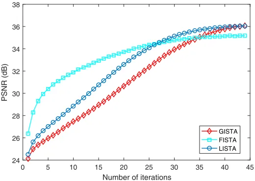
In this section, we compare PSNR changes in different algorithms as the number of iterations increases. The selected MR images are identical and are the third image of Fig. 2. In the parameter selection, we set J for each type of algorithm to 2, set the step size tk to 1, and set the regularization parameter λ to 1. The standard deviation of the added noise is 0.01. Record the recovery effect of each algorithm on the same graph as the number of iterations increases.
Figure 5 lists the PSNR values for various iterations. For various iterative threshold class algorithms, when the number of iterations is greater than 35, good results can be maintained under low noise conditions, but if the number of iterations is less than 30, various algorithms based on gradient descent cannot achieve good results. As can be seen from Fig. 5, our proposed LISTA algorithm outperforms other algorithms with a sufficient number of iterations. Although LISTA algorithm is not as accurate as the FISTA algorithm in the case of too few iterations, the number of iterations in MR image recovery is generally sufficient, so this problem is acceptable.
0 5 10 15 20 25 30 35 40 45
Number of iterations
24 26 28 30 32 34 36 38
PSNR (dB)
GISTA FISTA LISTA
5. CONCLUSIONS
This paper presents a new iterative threshold method based on log-sum algorithm for the first time. The new idea is embedded in two aspects: embedding log-sum norm regularization into the iterative threshold method; setting a new iterative threshold operator. In this paper, we demonstrate in detail the robustness of the algorithm compared to other algorithms. Experiments are performed to show the good results of our method. It can be clearly seen that the new iterative threshold algorithm has a significant improvement in some cases such as MR image recovery, compared to the Lp norm and the L1 norm. The algorithm also has some shortcomings, i.e., the algorithm performs poorly at low iterations, which is related to the mathematical properties of log-sum norm. The iterative threshold operator needs more accurate estimation. When we process signals in real life, we often have more than one iterations, so this problem can be ignored.
ACKNOWLEDGMENT
This paper is supported by the National Key Laboratory of Communication Anti-jamming Technology (No. 614210202030217).
REFERENCES
1. Daubechies, I., M. Defrise, and C. D. Mol, “An iterative thresholding algorithm for linear inverse problems with a sparsity constraint,” Communications on Pure and Applied Mathematics, Vol. 57, No. 11, 1413–1457, 2004.
2. Beck, A. and M. Teboulle, “A fast iterative shrinkage-thresholding algorithm for linear inverse problems,” SIAM Journal on Imaging Sciences, Vol. 2, No. 1, 183–202, 2009.
3. Bioucasdias, J. M. and M. A. Figueiredo, “A new twist: Two-step iterative shrinkage/thresholding algorithms for image restoration,”IEEE Transactions on Image Processing, Vol. 16, No. 12, 2992– 3004, 2007.
4. Zuo, W., et al., “A generalized iterated shrinkage algorithm for non-convex sparse coding,”
Proceedings of the IEEE International Conference on Computer Vision, 2013.
5. Wang, P., P. Duan, and S. Xiong, “Image deblurring via fast generalized iterative shrinkage thresholding algorithm for lp regularization,” Journal of Wuhan University (Natural Science Edition), 2017.
6. Chartrand, R. and W. Yin, “Iteratively reweighted algorithms for compressive sensing,”Acoustics, Speech and Signal Processing, 2008.
7. Zeng, J., et al., “Regularization: Convergence of iterative half thresholding algorithm,” IEEE Transactions on Signal Processing, Vol. 62, No. 9, 2317–2329, 2013.
8. Cho, S., J. Wang, and S. Lee, “Handling outliers in non-blind image deconvolution,” International
Conference on Computer Vision IEEE Computer Society, 2011.
9. Dong, J., et al., “Blind image deblurring with outlier handling,” IEEE International Conference
on Computer Vision (ICCV) IEEE, 2017.
10. Rostami, M., O. Michailovich, and Z. Wang, “Image deblurring using derivative compressed sensing for optical imaging application,” IEEE Transactions on Image Processing, Vol. 21, No. 7, 3139– 3139, 2012.
11. Yin, X., L. Wang, H. Yue, and J. Xiang, “A new non-convex regularized sparse reconstruction algorithm for compressed sensing magnetic resonance image recovery,”Progress In Electromagnetics Research C, Vol. 87, 241–253, 2018.
12. Rao, B. D. and K. Kreutz-Delgado, “An affine scaling methodology for best basis selection,” IEEE Transactions on Signal Processing, Vol. 47, No. 1, 187–200, 2002.
14. Deng, Y., et al., “Low-rank structure learning via log-sum heuristic recovery,” 5th Pacific Rim Conference on Multimedia, 1012–1919, Mathematics, 2010.
15. Candes, E. and T. Tao, “Near optimal signal recovery from random projections: Universal encoding strategies,” IEEE Trans. Inf. Theory, Vol. 52, No. 12, 5406–5425, 2006.