Nonlinear sem: Comparison between endogenous and exogenous interaction

Full Length Research Article

NONLINEAR SEM: COMPARISON BETWEEN ENDOGENOUS AND EXOGENOUS INTERACTION

*Gloria Gheno

Faculty of Economics and Management, Free University of Bozen-Bolzano, 39100 Bolzano

ARTICLE INFO ABSTRACT

In many fields of research to study particular phenomena the analysis of model with interaction is very important. The interaction occurs when the effect of a variable on another variable varies with the varying of a third variable and vice versa. In the SEM analysis the interaction can create problems if the two cause-variables are endogenous, i.e. linked causally to other variables. In literature, only few authors examined the model with the interaction between endogenous variables but without a true analysis of the causal effects. Consequently to analyze this particular model I propose two methods which link the causal theory to the mathematical relations used in the estimation process. The two methods use different causal theories then they consider the interaction in different way, the first as an exogenous variable and the second as an endogenous. To compare them, I analyze 4 groups of simulated datasets and , finding that the two methods give substantially the same results, for the simplicity I advise the use of the exogenous method.

Copyright©2016, Gloria Gheno. This is an open access article distributed under the Creative Commons Attribution License, which permits unrestricted use, distribution, and reproduction in any medium, provided the original work is properly cited.

INTRODUCTION

In literature, the causal analysis and the SEM methods (Structural equation model) are often analyzed in disjointed manner and developed separately even though initially the study of the causality originated from the structural part of the SEM models (Wright, 1921). The causal theory, in fact, mainly aiming to study in the theoretical models the cause-effect relationships among variables, proving its existence and measuring the intensity, very often does not deal with estimating them from real data. With the causal analysis, then, the researcher tries to define a relation between a cause variable and a effect variable, where the latter is interpreted as a consequence of the first. The mediation analysis can be used to study the relationships among multiple variables and to try to discover the causal pathways through which the variations are transmitted from the cause to the effect. In mediation, therefore, a variable affects another variable through other variables, called mediators. An example of causal theory applicable to all models, and in particular to the mediation analysis, can be that proposed by Pearl (1998, 2009, 2012, 2014), who analyzes several causal pathways and proposes rules to determine the causal effects, sometimes unidentifiable for the presence of the correlation or of particular variables. The correlation does not imply causation even if it measures

*Corresponding author: Gloria Gheno,

Faculty of Economics and Management, Free University of Bozen-Bolzano, 39100 Bolzano.

the strength of the link between two variables, in fact between two correlated variables a causal relationship may exist or not. Hayes and Preacher (Preacher and Hayes, 2008; Hayes and Preacher, 2010; Hayes, 2013) offer another example of causal theory, but it is only applicable to linear models, considering the problem of identification of the effects and studying primarily the phenomenon of the mediation and the moderation. They distinguish the mediation in series from that parallel. If a mediator causally influences another mediator, then the mediation presents mediators in series, if causally disjoint they become parallel. This analysis is also developed by Pearl who shows the cases in which the effects are identifiable. The moderation occurs, however, when the effect of a variable on another variable varies with the varying of a third variable, called moderator. Pearl does not consider the moderation, but a similar effect, called interaction, in which the effect of a cause variable on an effect variable depends on a third variable and vice versa. The structural equation models incorporate various statistical concepts, such as confirrnatory factor analysis, path analysis, multiple regressions, ANOVA and simultaneous equation models. The SEM presents a structural part, which defines the direct relationship among the unobserved variables, and a measurement part, in which the unobserved variables, or latent, are derived from the observed variables, called indicators (Bollen, 1989). The structural part and the causal diagrams (Wright, 1921) have an origin in common, while the measurement part mainly derives from the explanatory factor analysis (Spearman, 1904). The link

ISSN: 2230-9926

International Journal of Development Research

Vol. 06, Issue, 10, pp.9850-9857, October, 2016

DEVELOPMENT RESEARCH

Article History: Received 19th_{July, 2016} Received in revised form 28th_{August, 2016}

Accepted 20th_{September, 2016} Published online 31st_{October, 2016}

Key Words:

between Wright’s work and today's use of the SEM models

requires a clarification. Wright invented the analysis of the path diagram to estimate the effects when a pattern is known, the SEM, however, using the data to test a hypothesized model, can only invalidate a model but never confirm it (Kline, 2011). The measurement part and that structural were unified in the 70s by the work of Jöreskog, Keesling and Wiley. In its first statement, the structural part of the SEM, called linear SEM later, consists of a systems of linear-in-parameters and linear-in-variables equations. The variables are defined endogenous if obtained causally from other variables, exogenous all remaining. The endogenous variables, then, are linearly dependent on the exogenous variables, on the other endogenous variables and on the error term, which can be interpreted as a set of factors not considered in the model. The variables can be linked both causally and through the correlation, then, to find the parameters, SEM minimizes a function, called fitting function, of the distance between the matrix of variance-covariance implied in the theoretical model and the same matrix obtained from the data. Many different fitting functions are proposed, for example that used by the maximum likelihood method (ML) or that considered by the unweighted least squares method (ULS).

Later Kenny and Judd (1984) introduced the interaction in a structural equation model with latent variables, called nonlinear SEM with latent variables. This introduction transforms a model with the linearity in the parameters and in the variables into one with the linearity only in the parameters obtaining so a more complex model, and therefore applicable to more situations. In Kenny and Judd’s paper (1984) the

indicators of the nonlinear term are equal to the products of the various indicators of the two latent exogenous variables which form the interaction, making so possible its inclusion in the SEM. Many authors, afterwards, proposed various other types of indicators for the interaction (for example, Ping, 1995; Jöreskog and Yang, 1996; Marsh et al., 2004) or various other methods of estimation for the non-linear SEM (for example Bollen and Paxton, 1998; Henseler and Chin, 2010). The German school (Moosbrugger et al., 1997; Kelava et al., 2008; Moosbrugger et al., 2009; Brandt et al., 2014) analyzed the nonlinear SEM to improve its applicability to real data, considering both the indicators problem and that of the estimation process. For example, Klein and Moosbrugger (2000) propose a method which does not require the indicators for the latent interaction, being this calculated directly by the latent variables. In general all authors do not make a true causal analysis for the nonlinear SEM and they consider only the interaction between two exogenous variables.

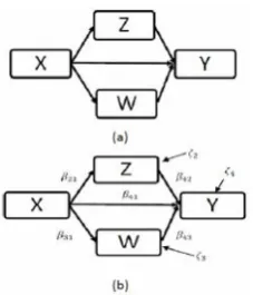
Figure 1. Mediation model with parallel mediators and with

uncorrelated errors according to Kenny and Judd’s path diagram (a) and according to SEM’s path diagram (b)

Only Coenders et al. (2008) and Chen and Cheng (2014) analyze the interaction between two endogenous variables, the first considering a mediation model with the interaction between the mediators in series, the second a mediation model with the interaction between the parallel mediators with uncorrelated errors. Coenders et al. (2008) propose an approximate causal analysis, estimating a different model from that used in their study. The lack of the causal analysis linked to an estimation method in a model with parallel mediators and interaction between endogenous variables, leads me to propose two new estimation methods and to compare them both in theoretical terms and in the applicative use. The two methods differ in the different applied causal theories and in the different estimated causal equations. In Section 1 and Section 2 I propose two new methods for a model with parallel mediators and for a model with parallel mediators and interaction. In Section 3, I apply the two methods, found in the previous sections, in simulated data to compare them under different assumptions.

A mediation model with parallel mediators

To find a method which examines together both the causal analysis and the estimation procedure, I consider the causal theories proposed by Pearl (2009, 2012, 2014) and by Hayes and Preacher (Preacher and Hayes, 2008; Hayes and Preacher, 2010; Hayes, 2013). Based on these or on their modifications, I reformulate the structural part of the SEM to make it applicable to it. Initially I analyze a simple mediation model with parallel mediators as that depicted in the path diagram of Fig. 1(a), where the variable X influences directly the two mediators Z and W. These three variables, in turn, influence the variable Y . The arrows represent the direct causal effect of one variable on another variable, not mediated by other variables. Assuming a SEM model, Figure 1(a) (Kenny and Judd, 1984) can be represented in more detail in Fig. 1(b) (Bollen, 1989), in which the error terms are inserted. The lack of double arrow between the two terms of the mediators error,

ζ and ζ , involves their uncorrelation. The coefficients β

quantify the direct effect of a variable on another variable. In SEM terminology, therefore, the variable X is called exogenous because it is not influenced by any other variable, while the variables Z, W and Y are called endogenous, because they are affected by other variables. For example, the variable Z is influenced by the variable X and quantifies its effect. Only under the four conditions proposed by Mulaik (2000), and taken up again by Kline (2011), the direct effects estimated by the SEM model, i.e. the parameters β, can

measure the causality. In this simple case nothing of the structural part of SEM must be modified to be able to apply the two causal theories to the path diagram. The first method,

using Pearl’s concepts, calculates the effects considering any

variation of X (Δ X) and one mediator at a time. As a result, I

have two groups of causal effects depending on which mediator is used. Considering as mediator the variable Z, the effects proposed by Pearl are:

⎩ ⎪ ⎨ ⎪

⎧ , ′= ( ′, ) − ( | , ) ( | )

, ′= ( | , ) ( ′), ( | )

, ′ = , ′, ′_,

DE, is the effect of X on the endogenous variable Y without considering the effect mediated by the variable Z. The indirect effect, IE, is the effect of variable X on Y only through the variable Z and the total effect (TE) is equal to the direct effect minus the indirect effect of the inverse variation of X. In the linear case, because ′ is equal to− _, ′, it is still true the

traditional decomposition of the total effect in direct effect and indirect effect. Now I apply these formulas to the simple model with parallel and uncorrelated mediators to complicate it successively in order to make it applicable to more real cases. Initially I consider Z as mediator and I note that the effect of the other mediator W is inserted in the direct effect:

Mediator Z

= ( + )∆

= ( )∆

= ( + + )∆

The parameter is the direct effect of X on Y, the product the indirect effect of X on Y through the mediator W and the product the indirect effect of X on Y through Z. The total effect is equal to the sum of direct and indirect effects because the relationship is linear. The causal effects for the mediator W are:

Mediator W

= ( + )∆

= ( )∆

= ( + + )∆

From these equations it is clear that in Pearl’s theory the

effects are a function of the variation. To simplify the interpretation of these effects and to make them comparable with those obtained by other methods, I consider the rate at which the value of the variable Y changes as regard the

change of variable X (ΔY / ΔX). In the linear case, I get so that

the effects in the rate version are no longer a function of the change. For example, the direct effect becomes equal to

+ . If I want to examine the instant version, so that the effects are not a function of the variation of X also in the nonlinear case, I calculate the limit of the ratio with x which goes to ′_{. In this case, because the relationships are linear, the}

instantaneous version and the ratio are equal. Now I analyze my second method, which uses the causal theory proposed by Hayes and Preacher. Their effects are the instantaneous

version of the ratio ΔY / ΔX and are therefore not a function of

the variation of X. They consider the mediators together and then they propose in addition to the specific indirect effects of the individual mediators (SIE (Z) and SIE (W)) the total indirect effect, which considers them together. The effects then become:

= =

( )

+

( )

= + +

I conclude, therefore, that my two methods give essentially the same results, since the only difference is due to the role of second mediator and to the change of the exogenous variable X. If in Pearl’s theory I consider the ratio ΔY/ΔX and the

mediators together, then I obtain exactly Hayes and

Preacher’s causal effects. Now I complicate the previous model adding the correlation between the errors of the variables Z and W to remove a further limitation to its

application. The method which uses Hayes and Preacher’s

theory remains unchanged, while that which applies Pearl’s theory has some limitations. Pearl’s theory, in fact, being

applicable to any type of model (parametric, non-parametric, etc.) requires that the parallel mediators have uncorrelated errors. I therefore propose new formulas for calculating the effects

⎩ ⎪ ⎪ ⎪ ⎨ ⎪ ⎪ ⎪

⎧ , ′= ( ′, , ) − ( | , , )

, ,

( , | , , ) ( , )

, ′ = ( | , , )

, ,

( , ′_{, , ) − ( , | , , )}

, , ′= , ′− ′_,

where I consider together the mediators and I analyze the effects of the error terms ζ andζ of the mediators. Of course, these formulas may also be applied to the previous parallel mediation model without correlated errors or to particular nonparametric models. The causal effects with the first method become

= ∆

= ( + )∆

= ( + + )∆

I define these effects as modifications to Pearl’s theory. The direct effect becomes that produced directly only by the exogenous variable X, while the indirect effect is due both to the mediator Z ( ) and to the mediator W ( ). The total effect is still equal to the sum of the direct and indirect effects. In this case, the two methods provide substantially the same results, since the only difference is due to the variation of the exogenous variable X. If I consider the instantaneous version of the effects of the modified theory proposed by Pearl, I get exactly Hayes and Preacher’s effects. The

introduction of covariance does not influence the technique of the second method, but only that of the first, but it does not modify substantially the results of both. The proposed estimation procedure for the two methods is the maximum likelihood (ML), typical for the SEM. The variance-covariance matrix of the model is obtained from the regressions described in the path diagram of Fig. 1(b) when the mediators are uncorrelated and those of the same plot, but adding the correlation when the mediators are correlated. The variables X, Z and W are normally distributed with zero mean. The errors of mediators Z and W, ζ andζ , are distributed as a multivariate normal with the mean vector equal to the zero vector, with the variances equal to and and with the covariance between the errors of the two mediators equal to . In the simplest case, the covariance is equal to 0, and then, for the property of multinormal variables, the errors ζ

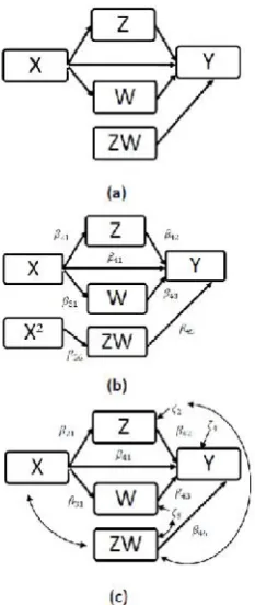
Figure 2. Mediation model with parallel mediators and with uncorrelated errors, according to Kenny and Judd (a), with X² (b) and according to the first method (c)

The estimation procedure in the presence of latent variables, however, changes because it is necessary to introduce the linear relationships between the observed variables and latent ones, to derive the latter. The implied variance-covariance matrix, then, is obtained considering both the causal regressions and the relations between the latent variables and those observed. Using the same estimation procedure for both methods and giving the causal theory essentially the same results, in the linear SEM the use of this or of that method is indifferent.

A parallel mediation model with interaction

Introducing the interaction term between the endogenous variables Z and W, I complicate further the path diagram of Fig. 1(a) so that the direct effect of a mediator depends on the other. The new path diagram, free from assumptions on the implicit model, is shown in Fig. 2(a), in which the interaction is introduced by the product ZW, which influences the variable Y. In this case the interaction, being obtained by the product between two endogenous variables, becomes an endogenous variable. Assuming a nonlinear model it is correct to insert an arrow going from X to ZW, but under the hypothesis of linearity of the model this introduction cannot be done and Fig. 2(a) is then correctly replaced by Fig. 2(b). To start from the simplest model I take into consideration the model with the error terms of Z and W not correlated and I apply to it my two methods.The first method uses Pearl’s theory. The author in

his paper introduces the interaction, analyzing, however, only that obtained by the product of an exogenous variable and an endogenous variable. His causal theory uses the distribution of the variables to calculate the effects and not the relations formulated in the regressions which determine the endogeneity or the exogeneity of the variables. As a result I can estimate this model recalling that in the estimation process proposed by Coenders et al (2008) and Chen and Cheng (2014), the

interaction is considered exogenous even though in reality it is endogenous. The ZW interaction, then, is linked to the variables Z, W and X only through the covariances Cov (ZW,

ζ ), Cov (ZW,ζ ) and Cov (ZW, X) as shown in Fig. 2(c). The direct, indirect and total effects for the mediator Z and for the mediator W are respectively

Z:

= ( + + )∆

= ( + )∆

= ( + + )∆ + ∆

W:

= ( + + )∆

= ( + )∆

= ( + + )∆ + ∆

As for the model without interaction, the indirect effect through the variable W becomes a part of the direct effect if Z is the mediator, while the indirect effect through the variable Z becomes a part of the direct effect if W is the mediator. The introduction of the interaction inserts the same part of the effect ΔX both in the direct effect and in the indirect effect. The total effect is not equal to the sum of the direct and indirect effects when the relationships are not linear, as noted by Pearl (2012). If I consider the relationship to eliminate the variation of the variable X, I obtain that the direct and indirect effects become a function of the initial value of X, i.e. , while the total effect becomes a function of the sum of the initial value and of the final value ′_{. The}

instantaneous variation does not affect the indirect and direct effects obtained from the ratio, but it changes the total effect

which becomes + + + 2 . The

indicator can be multiplied only one time. Of course, to eliminate the means structure, it is necessary also to center the indicators of the interaction. These indicators are called double mean centered indicators and are proposed by Lin, Wen, Marsh and Lin (2010). The second method uses Hayes and

Preacher’s theory. As already stated in the introduction, they

do not consider the interaction but only the moderation and therefore I am not able to use their causal theory for this effect. I apply to the interaction the causal theory which they propose when the mediator is a function (Preacher and Hayes, 2010), i.e., for example, when X influences directly and linearly Z and only a function of Z, defined F (Z), influences Y. In this case the indirect effect is equal to = ( ⁄ )( ⁄ ), where the first multiplier calculates the causal effect of Z on Y and the second the causal effect of X on Z. Hayes and

Preacher’s theory, unlike that proposed by Pearl, uses only the

relations of the regressions to calculate the effects and therefore it requires that in the model there is a covariance between Z and F (Z) so that there is also a causal relationship between X and F (Z). In the method proposed by Coenders et

al. (2008) and by Chen and Cheng (2014) the correlation

between F(Z) and Z is not present because it is the term error of Z which correlates with F (Z), and then F (Z ) and X are not causally linked. In the traditional SEM, even if there is a causal relationship between X and Z and between F (Z) and Y, the correlation between F (Z) and Z there is not, as shown in Fig. 2 (c). The correlation between Z and F (Z) is present, instead, in the estimation process proposed by Klein and

Moosbrugger (2000), and then Hayes Preacher’s theory can be

used without modifications. I underline, however, that the same causal authors do not consider this problem in the estimation process.

To connect, therefore, causally the interaction term ZW and the exogenous variable X, I introduce this regression

= ( − ( )) +

= ( − ( )) +

such that I solve this limitation. With this introduction I formulate the model shown in Fig.2 (b). The variables X and X² are correlated and X² influences causally ZW. The variable X causally influences the interaction ZW so I can use the formula proposed by Hayes and Preacher (2010). I center X² to eliminate the means structure, as already explained for the first method, in fact, if X² is centered, also ZW and Y are centered. The causal effects, taken together the two mediators, thus become

=

= + + 2

= + + + 2

The direct effect remains equal to that of the model without interaction. The same part of effect2 is added to the indirect effect and the total effect. The parameter is obtained from the partial derivative of Y on ZW, while the product 2 is obtained from the partial derivative of ZW on X. These effects are substantially similar to those obtained with the first method analyzing together the mediators and the instantaneous variation of the ratio. I use the same estimation procedure of the first method, but in this case X remains an exogenous variable, Z, W and Y remain endogenous variables and ZW becomes an endogenous variable. In this way, I consider the interaction between

endogenous variables as endogenous, unlike Coenders et al (2008) and Chen and Cheng (2014). The interaction ZW is related to the variables Z and W only through the covariances Cov ( , ζ ) and Cov ( , ζ ), while it is linked to X only through the causal relationship with X². If the variable X, Z,W and Y are not observed, the problem is solved as in the exogenous method and the difference is in the introduction of the indicators for X². I advise also for X² the double mean centered indicators proposed by Lin, Wen, Marsh and Lin (2010). The introduction of the interaction causes a difference between the regressions of the two methods, due to the different treatment of the variable ZW. For this reason I call the first method "exogenous interaction" and the second method "endogenous interaction". Now I complicate further the model of Fig. 2(a) adding the correlation between the error terms of the mediators Z and W. The first method, called exogenous interaction, requires the use of modified Pearl’s

theory in which the two mediators Z and W are considered together. The causal effects then become

=

= ( + )∆ + ∆

= ( + + )∆ + ∆

The direct effect is a function of the variation of X, while the indirect effect and the total effect are a function of the variation of X, of the initial value and of the final value ′. If I consider together both the ratio and the instantaneous variation, the direct effect becomes a constant, while the indirect effect and the total effect become only a function of the initial value , in fact, the indirect effect with the

instantaneous variation is + + +

2 . The introduction of the correlation in a parallel mediation model with interaction causes the impossibility of considering separately the two mediators. The estimation process remains the same as that proposed for the parallel model with interaction and without the correlation between the error terms of Z and W, i.e. the MLMV method. The second method, also called endogenous interaction, does not require modifications when the correlation is introduced, then the effects and the estimation procedure remain equal to those calculated for parallel model without the correlation between the error terms of Z and W. Summarizing, if I introduce the correlation, the exogenous method, or first method, is no longer able to calculate the effects considering separately the two mediators, while the endogenous method, or second method, is not affected by this introduction. If the interaction is added, the endogenous method is no longer able to calculate the causal effects from regressions, then it is necessary to add a new regression to endogenize the interaction term, while the exogenous method is not affected by this introduction. The two methods give essentially the same results under the four proposed theoretical models. I recommend the use of the exogenous interaction method being simpler than the other because it does not require the introduction of a new regression. The transition from variables observed to latent variables is the same in both methods.

Applications

groups are different from each other only for the value of the covariance between the errors of the mediators. The estimation method is the same in both methods because I analyze a parallel mediation model without interaction. The results are reported in Table 1. In the first column there is the true value

of the parameters β, in the third, fourth, fifth and sixth column

for any parameter there are the estimated values, the powers and the 95% coverage indices in 4 different groups of datasets, which differ only in the covariance. The power of the parameter is measured as the ratio between the number of datasets, in which the parameter is significant, and the total number of datasets. According to Bradley (1978), a value between 0.025 and 0.075 corresponds to a parameter equal to 0. According to Thoemmes et al. (2010), the power must be greater than 0.8 for the parameters different from 0. The 95% coverage index is the percentage of times in which the value of the population is included in the confidence interval of the estimated parameters. According to Muthén and Muthén (2002) this index must be greater than 0.91 and less than 0.98. According to Collins, Kam and Schafer (2001), this index must be greater than 0.90. The powers of the parameters in the model are all larger than 0.8 with the exception of that of the parameter , which in the dataset with negative covariance is equal to 0.6. This result is due to the problem of a low R², as noted by Grewal et al. (2004). Being all positive parameters, in fact, a decrease of the covariance causes a decrease of the R² with probable problems of the power. The 95% coverage index, however, is always greater than 0.91. These indices indicate that the methods give good estimates and that the covariance influences the power but not the 95% coverage index.

Table 1. Parameters estimated in a parallel mediation model, E = estimated value, P = power and C = 95% convergence index

Dataset with = 0.4 0.13 0 -0.4

E 0.3994 0.1291 -0.0010 -0.4010

P 1.000 1.000 0.056 1.000

C 0.958 0.941 0.944 0.944

= 0.63

E 0.6323 0.6322 0.6320 0.6305

P 1.000 1.000 1.000 1.000

C 0.954 0.957 0.950 0.940

= 0.77

E 0.7712 0.7702 0.7701 0.7709

P 1.000 1.000 1.000 1.000

C 0.947 0.945 0.944 0.934

= 0.27

E 0.2713 0.2713 0.2714 0.2716

P 0.956 0.946 0.924 0.605

C 0.952 0.951 0.949 0.951

= 0.45

E 0.4490 0.4495 0.4495 0.4494

P 1.000 1.000 1.000 1.000

C 0.949 0.947 0.946 0.947

= 0.57

E 0.5707 0.5703 0.5703 0.5698

P 1.000 1.000 1.000 1.000

C 0.960 0.963 0.964 0.954

The causal effects obtained with the first method and with the

two mediators considered together are: DE = 0.27ΔX, IE = 0.7224ΔX and TE = 0.9924ΔX. The causal effects obtained

with the second method are: DE = 0.27, SIE (Z) = 0.2835, SIE (W) = 0.4389, IE= 0.7224 and TE = 0.9924. If I consider the effects obtained with the first method with the analysis of the variation of Y with respect to the variation of X, the first method gives the same results of the second. Now I introduce the interaction term to analyze the methods modified as in the third section. I examine the four groups of datasets simulated by a parallel mediation model with interaction and with observed variables.

Table 2. Estimated parameters in a parallel mediation model interactively, exogenous method, E=estimated values,

P = power and C = 95% coverage index

Dataset with = 0.4 0.13 0 -0.4

E 0.3991 0.1293 0.0000 -0.3997 P 1.000 0.999 0.051 1.000 C 0.953 0.948 0.949 0.954 =0.63 E 0.6305 0.6315 0.6292 0.6317

P 1.000 1.000 1.000 1.000 C 0.958 0.947 0.963 0.942 =0.77 E 0.7693 0.7693 0.7702 0.7693

P 1.000 1.000 1.000 1.000 C 0.951 0.951 0.943 0.951 =0.27 E 0.2697 0.2691 0.2691 0.2671

P 0.943 0.940 0.923 0.575 C 0.945 0.960 0.952 0.960 =0.45 E 0.4523 0.4514 0.4504 0.4522

P 1.000 1.000 1.000 1.000 C 0.953 0.953 0.937 0.951 =0.57 E 0.5684 0.5700 0.5692 0.5722

P 1.000 1.000 1.000 1.000 C 0.945 0.941 0.937 0.954 =0.23 E 0.2304 0.2309 0.2276 0.2311

P 1.000 0.996 0.990 0.996 C 0.946 0.950 0.945 0.937

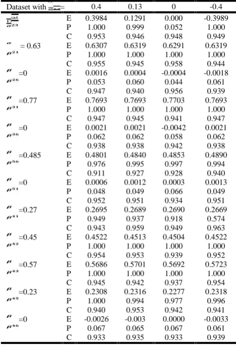
Table 3. Parameters estimated in a parallel mediation model with interaction, endogenous method, E=estimated values, P = power

and C = 95% coverage index

Dataset with = 0.4 0.13 0 -0.4

E 0.3984 0.1291 0.000 -0.3989 P 1.000 0.999 0.052 1.000 C 0.953 0.946 0.948 0.949 = 0.63 E 0.6307 0.6319 0.6291 0.6319

P 1.000 1.000 1.000 1.000 C 0.955 0.945 0.958 0.944 =0 E 0.0016 0.0004 -0.0004 -0.0018

P 0.053 0.060 0.044 0.061 C 0.947 0.940 0.956 0.939 =0.77 E 0.7693 0.7693 0.7703 0.7693

P 1.000 1.000 1.000 1.000 C 0.947 0.945 0.941 0.947 =0 E 0.0021 0.0021 -0.0042 0.0021

P 0.062 0.062 0.058 0.062 C 0.938 0.938 0.942 0.938 =0.485 E 0.4801 0.4840 0.4853 0.4890

P 0.976 0.995 0.997 0.994 C 0.911 0.927 0.928 0.940

=0 E 0.0006 0.0012 0.0003 0.0013

P 0.048 0.049 0.066 0.049 C 0.952 0.951 0.934 0.951 =0.27 E 0.2695 0.2689 0.2690 0.2669

P 0.949 0.937 0.918 0.574 C 0.943 0.959 0.949 0.963 =0.45 E 0.4522 0.4513 0.4504 0.4522

P 1.000 1.000 1.000 1.000 C 0.954 0.953 0.939 0.952 =0.57 E 0.5686 0.5701 0.5692 0.5723

P 1.000 1.000 1.000 1.000 C 0.945 0.942 0.937 0.954 =0.23 E 0.2308 0.2316 0.2277 0.2318

P 1.000 0.994 0.977 0.996 C 0.940 0.953 0.942 0.941 =0 E -0.0026 -0.003 0.0000 -0.0033

P 0.067 0.065 0.067 0.061 C 0.933 0.935 0.933 0.939

endogenous, it is necessary to add a new regression in which the interaction ZW is given by the variable X². I examine the introduction of the variable X² inserting it as regressor in the regressions of Z, W and Y with the parameters , and . To perform the same control, I introduce X as regressor in the regression of the interaction ZW with the parameter . If the estimates are correct, the parameters , , and should not be significant. The estimated parameters are given in Table 2 and in Table 3. In both methods, the 95% coverage indices are good, and the powers of the parameters are greater than 0.8, except that of the parameter in the datasets with negative covariance. This result is due to the low value of R², as noted by Grewel et al. (2004). The power of the parameters, which are not present in the true model, are all smaller than 0.075 and this is coherent with a parameter equal to 0. With the analysis of the two indices, I testify that both methods, both that with exogenous interaction and that with endogenous interaction, give good estimates. For its simplicity, I suggest the use of the exogenous method. The causal effects obtained with the first method and with the two mediators considered

together are: DE = 0.27ΔX, IE = 0.7224ΔX + 0.111573ΔX² and TE = 0.9924 ΔX+ 0.111573 ΔX². The causal effects

obtained with the second method are: DE = 0.27, IE = 0.7224 + 0.223146 and TE = 0.9924 + 0.223146 . I underline that the effects obtained with the first method, analyzing the variation of Y with respect to the instantaneous variation of X, are equal to those of the second.

DISCUSSION

In this article, I propose two methods which consider both the causal analysis and the estimation process in a model with parallel mediators to solve the problem of interaction between

endogenous variables. The first method uses Pearl’s theory, or

his version modified by me, and it estimates the regressions in which the dependent variables are only Z, W and Y. The

second method, instead, follows Hayes and Preacher’s theory

using regressions which have the variables Z, W, Y and the interaction ZW as dependent variables. I insert the interaction ZW as dependent variable to be able to link it causally to the variable X so that I can apply to the model the causal theory proposed by Hayes and Preacher. I examine initially a parallel mediation model without interaction. The two methods have the same regressions and consequently also the same estimation process. If I consider a parallel mediation model with interaction term, the first method, also called exogenous, continues to use the same regressions of the model without interaction. The second method, called endogenous, introduces, instead, the regression in order that ZW becomes a dependent variable. The endogenous and exogenous methods estimate different models in the estimation process. To investigate which method have a better application, I compare the two methods using simulated datasets. The analysis shows that both methods give good results. I advise, therefore, the use of the first method for its simplicity because the causal analysis and the estimation process substantially give the same results.

REFERENCES

Bollen, K. A. 1989. Structural equations with latent variables. John Wiley and Sons, N.Y.

Bollen, K. A., and Paxton, P. 1998. Interaction of latent variables in structural equation models. Structural equation

modeling: A Multidisciplinary Journal, vol. 5(3), pp

267-293

Bradley, J. V. 1978. Robustness?, British Journal of

Mathematical and Statistical Psychology, vol. 31(2), pp

144-152

Brandt, H., Kelava, A. and Klein, A. 2014. A simulation study comparing recent approaches for the estimation of nonlinear effect in SEM under the conditional nonnormality, Structuarl equation modeling: A Multidisciplinary Journal, vol. 21, pp 181-195

Chen, S-P, and Cheng, C-P. 2014. Model specification for latent interactive and quadratic effects in matrix form, Structural equation modeling: A Multidisciplinary Journal, vol. 21, pp 94-101

Coenders, G., Batista-Foguet, J. M., Saris, W. E. 2008. Simple, efficient and distribution-free approach to interaction effects in complex structural equation models, Quality and Quantity, vol. 42, pp 369-396

Collins, L. M, Schafer, J. L., and Kam, C-M 2001. A comparison of inclusive and restrictive strategies in modern missing data procedures, Psychological methods, vol. 6(4), pp 330-351

Grewal, R., Cote, J. A., and Baumgartner, H. 2004. Multicollinearity and measurement error in structural equation models: implications for theory testing, Marketing

Sciences, vol.23(4), pp 519-529

Hayes, A. F. 2013. Introduction to mediation, moderation and conditional process analysis: a regression-based approach, The Guilford press, N.Y.

Hayes, A. F., and Preacher, K. J. 2010. Quantifying and testing indirect effects in simple mediation models when the constituent paths are nonlinear, Multivariate Behavioral

Research, vol. 45, pp 627-660

Henseler, J., and Chin, W.W., 2010. A comparison of approaches for the analysis of interaction effects between latent variables using partial least squares path modeling, Structural equation modeling: A Multidisciplinary Journal, vol. 17(1), pp 82-109

Jöreskog, K. G. and Yang, F. 1996. Nonlinear structural equation models: The Kenny-Judd model with interaction effects. In G. A. Marcoulides andR. E. Schumacker (Eds.) Advanced structural equation modeling techniques (pp. 57-88). Hillsdale, NJ: Lawrence Erlbaum.

Kelava, A., Moosbrugger, H., Dimitruk, P. and Schermelleh-Engel, K. 2008. Multicollinearity and missing constraints,

Methodology, vol.4(2), pp 51-66

Kenny, D, A. and Judd. C. M. 1984. Estimating the nonlinear and interactive effects of latent variables. Psychological

Bulletin, vol. 96, pp 201-210

Kline, R. 201). Principles and practice of structural equation models. The Guilford press, N.Y.

Lin, G. C., Wen, Z., Marsh, H. W. and Lin, H. S. 2010. Structural equation models of latent interactions: Clarification of orthogonalizing and double-mean-centering strategies, Structural Equation Modeling, Vol. 17,pp 374-391

Marsh, H. W.,Wen, Z and Hau, K. T. 2004. Structural equation models of latent interactions: evaluation of alternative estimation strategies and indicator construction,

Psychological Methods, vol. 9, pp 275-300

Moosbrugger, H. and Klein, A. 2000. Maximum likelihood estimation of latent interaction effects with the LMS method, Psychometrika, vol. 65(4), pp 457-474

effects, Methods of Psychological Research Online, vol. 2(2)

Moosbrugger, H., Schermelleh-Engel, K., Keleva, A. and Klein, A. 2009. Testing multiple nonlinear effects in structural equation modeling: a comparison of alternative estimation approaches, chapter in T. Teo and M. S. Khine (Eds), Structural equation modelling in educational research: concepts and application. Rotterdam, NL: Sense Publishers.

Muthén, L. K., and Muthén, B. 2002. How to use a montecarlo study to decide on sample size and determine power, Structural equation modeling: A Multidisciplinary Journal, vol.9(4), pp 599-620

Pearl, J. 1998. Graphs, causality, and structural equation models, Sociological Methods and Research, vol. 27,pp 226-284

Pearl, J. 2009. Causal inference in statistics: an overview,

Statistical Survey, vol. 3, pp 96-146

Pearl, J. 2012. The mediation formula: A guide to the assessment of causal pathways in nonlinear models, chapter in Berzuini C., Dawid P. and Bernardinelli L. (Eds), Causality: Statistical perspectives and application, Wiley

Pearl, J. 2014. Interpretation and identification of causal mediation, forthcoming, Psychological Methods, vol

19,459-481

Ping, R. A. 1995. A parsimonious estimating technique for interaction and quadratic latent variables. Journal of

Marketing Research, vol. 32, pp 336-347.

Preacher, K. J. and Hayes, A. F. 2008. Asymptotic and resampling strategies for assessing and comparing indirect effects in multiple mediator models, Behavior Research

Methods, vol. 40 (3), pp 879-891

Satorra, A. and Bentler, P. M. 1994. Corrections to test statistics and standard errors in covariance structure analysis, chapter in A. Von Eye and C. Clogg (Eds), Latent variables analysis: applications to developmental research. Thousand Oaks, CA: Sage, pp 399-419

Spearman, C. 1904. General intelligence, objectively determined and measured. American Journal of Psychology, 15, pp. 201-293.

Thoemmes, F., Mackinnon, D. P., and Raiser, M. R. 2010. Power analysis for complex mediational designs using montecarlo methods, Structural Equation Modeling, Vol. 17(3), pp. 510-534

Wright, S. 1921. Correlation and causation. Journal of

Agricultural Research, 20(7), pp. 557-585.