Performance Evaluation of Image Retrieval using Co occurrence Matrix & Texton Co Occurrence Matrix

Volume 2, No. 6, Nov-Dec 2011

International Journal of Advanced Research in Computer Science REVIEW ARTICLE

Available Online at www.ijarcs.info

ISSN No. 0976-5697

Performance Evaluation of Image Retrieval using occurrence Matrix & Texton

Co-Occurrence Matrix

Sunita P. Aware* Department of VLSI. G.H.Raisoni College of Engineering,

Nagpur. (MS), India [email protected]

Laxaman P. Thakare Department of VLSI G.H.Raisoni College of Engineering,

Nagpur. (MS), India [email protected]

Abstract: This paper put forward a new method of co-occurrence matrix to describe image features. This method can express the spatial correlation of textons. During the course of feature extracting, we have quantized the original images into 256 colors and computed color gradient from the RGB vector space, and then calculated the statistical information of textons to describe image features. Image identification experimental results have shown that our proposed method has the discrimination power of color, texture and shape features, the performances are better than that of Grey Level Co-occurrence Matrix (GLCM) and Color Correlograms (CCG).

Keywords: Imaging and image processing co-occrrence matrix, texton matrix

I. INTRODUCTION

Object identification is one of the main topics in the field of computer vision and pattern recognition. In the early 1990s, researchers have built many objects identification systems, such as QIBC, MARS, and FIDS and so on. They are different from the traditional retrieval systems. These systems are based on image features such as color, texture, shape of objects and so on.

Nowadays, the main research work of image retrieval consists of feature extracting techniques, image similarly match and image identification methods.

Many researchers have put forward various algorithms to extract color, texture and shape features.

Color is the [1] most dominant and distinguishing visual feature. Color histogram-based techniques remain popular due to their simplicity, but it lacks spatial information. Several color descriptors try to incorporate spatial information to varying degrees, it include the compact color moments, color coherence vector and color correlograms.

Texture is used to specify the roughness or coarseness of object surface and described as a pattern with some kind of regularity. Many researchers have put forward various algorithms for texture analysis, such as the gray co-occurrence matrixes, Markov random field (MRF) model, simultaneous auto- regressive (SAR) model, World decomposition model, Gabor filtering and wavelet decomposition and so on.

Shape features are widely used in various areas such as object identification and content-based image retrieval. The classic method of describing shape features are moment invariants, Fourier transform Coefficients, edge curvature and arc length.

In order to integrate color, texture and shape features, this paper put forward a new method of co-occurrence matrix to describe image features. This method can express the spatial correlation of textons.

During the course of feature extracting, we have quantized the original images into 256 colors and computed color gradient from the RGB vector space, and then

calculated the statistical information of textons to describe image features.

Object identification experimental results have shown that our proposed method has the discrimination power of color, texture and shape features, the performances are better than that of GLCM and CCG. The paper is contained the gray occurrence matrix, the texton [2,7] co-occurrence matrix (TCM) and techniques of color edge extracting. The object identification performance resulted from GLCM, CCG. And our proposed method is compared by conducting two experiments over the Vistex texture database of MIT, Corel images and those images which come from web and concludes the paper.

II. METHODOLOGY

A. Description of co-occurrence matrix:

Suppose an image to be analyzed is rectangular and has Nx. resolution cells in the horizontal direction and Ny resolution cells in the vertical direction. Suppose that the gray tone appearing in each resolution cell is quantized to Ng levels.

Let Lx = {1,2,……,Nx} be the horizontal spatial domain, Ly = {1,2,…….,Ny} be the vertical spatial domain, and G = {1,2, …,Ng } be the set of Ng quantized gray tones. The set Ly X Lx is the set of resolution cells of the image ordered by their row-column designations.

The image I can be represented as a function which assigns some gray tone in G to each resolution cell or pair of coordinates in Ly X Lx; I: Ly X Lx =>G.

An essential component of our conceptual framework of texture is a measure, or more precisely, four closely related measures from which all of our texture features are derived. These measures are arrays termed angular nearest-neighbor gray-tone spatial-dependence matrices, and to describe these arrays we must emphasize our notion of adjacent or nearest-neighbor resolution cells themselves. We consider a resolution cell-excluding those on the periphery of an image, etc.to have eight nearest-neighbor resolution cells.

Sunita P. Aware et al, International Journal of Advanced Research in Computer Science, 2 (6), Nov –Dec, 2011, 199-203

relationship which the gray tones in image I have to one another. More specifically, we shall assume that this texture context information is adequately specified by the matrix of relative frequencies Pij with which two neighboring resolution cells separated by distance „d‟ occur on the image, one with gray tone i and the other with gray tone j. Such matrices of gray-tone spatial-dependence frequencies are a function of the angular relationship between the neighboring resolution cells as well as a function of the distance between them. The set of all horizontal neighboring resolution cells separated by distance 1. This set, along with the image gray tones, would be used to calculate a distance 1 horizontal gray-tone spatial-dependence matrix. Formally, for angles quantized to 450 intervals the un normalized frequencies aredefined as follows

P(i,j,d,00) = #{((k ,l),(m,n)) € (Ly x Lx) x (Ly x Lx) |k-m|= 0,|1 –n| =d, I(k,l) = i, I(m,n) = il

P(i,j,d,450) = #{((k ,l),(m,n)) € (Ly x Lx) x (Ly x Lx)I( k-m = d, l -n =-d) Or (k - m = -d, l - n =d), I (k, l) = i, I (m, n) = j P(i,j,d,900) = #{((k,l),(m,n)) € (Ly x Lx) x (Ly x Lx) | k- m| = d,|l-n|=0 I(k,l)=i,I(m,n)=j}

P(i,j,d,1350) = #{((k,l),(m,n)) e (Ly x Lx) x (Ly x Lx) (k - m = d, l- n = d) Or (k-m = -d, l-n= -d),

I (k, l) = i, I(m,n) = j} (1)

Where # denotes the number of elements in the set. Note that these matrices are symmetric;

P (i, j; d, a) = P (j, i; d, a). The distance metric p implicit in the preceding equations can be explicitly defined by P ((k, l), (m, n)) = max {|k – m|, |1- n|}.

B. Grey-level co-occurrence matrix texture:

Grey-Level Co-occurrence Matrix texture measurements have been the workhorse of image texture since they were proposed by Haralick in the 1970s. To many image analysts, they are a button you push in the software that yields a band whose use improves classification – or not.

The original works are necessarily condensed and mathematical, making the process difficult to understand for the student or front-line image analyst.

Calculate the selected Feature. This calculation uses only the values in the GLCM. See:

i) Contrast ii) Correlation iii) Energy iv) Homogeneity

These features are calculated with distance 1 and angle 0, 45 and 90 degrees. 2.3 K-Means Clustering

A cluster is a collection of data objects that are similar to one another with in the same cluster and are dissimilar to the objects in the other clusters. It is the best suited for data mining because of its efficiency in processing large data sets. It is defined as follows:

The k-means algorithm is built upon four basic operations:

a. Selection of the initial k-means for k-clusters.

b. Calculation of the dissimilarity between an object and the mean of a cluster.

c. Allocation of an object of the cluster whose mean is nearest to the object.

d. Re-calculation of the mean of a cluster from the object allocated to it so that the intra cluster dissimilarity is minimized.

The advantage of K-means algorithm is that it works well when clusters are not well separated from each other, which is frequently encountered in images.

C. Textural Features extracted from co-occurrence

matrices:

Our initial assumption in characterizing image texture is that all the texture information is contained in the gray-tone spatial-dependence matrices. Hence all the textural features we suggest are extracted from these gray-tone spatial-dependence matrices. Some of these measures relate to specific textural characteristics of the image such as homogeneity, contrast, and the presence of organized structure within the image. Other measures characterize the complexity and nature of gray tone transitions which occur in the image. Even though these features contain information about the textural characteristics of the image, it is hard to identify which specific textural characteristic is represented by each of these features. For illustrative purposes, we will define 3 of the 14 textural features in this section and explain the significance of these features in terms of the kind of values they take on for two images of distinctly different textural characteristics the features we consider are as follows

D. Textural Features:

a. Angular Second Moment: b. Contrast:

c. Correlation:

d. Sum of Squares: Variance: e. Inverse Difference Moment: f. Sum Average:

g. Sum Variance: h. Sum Entropy: i. Entropy:

j. Difference Variance: k. Difference Entropy:

Usually the neighboring pixels in an image are not very distinct (i.e. they are highly correlated). Quite often in an image there are large regions of pixels with nearly the same color, such as the sky, or with uniform texture, such as walls, cloth, or sand. For typical pixel-level texture feature extraction, the texture values for each pixel are computed with the sliding window positioned such that the pixel is the center of the window. Clearly, for images of the type mentioned above, the neighboring pixels have the same (or nearly the same) texture features. In such cases, nearly identical results are generated by performing nearly identical computations. If we can determine beforehand which computations will result in nearly identical results, we can avoid these calculations, trading off decreased computational complexity with a small amount of distortion in the texture extraction results.

We propose a new hierarchical method to reduce the computation complexity and expedite texture feature extraction according to this principle. In our method, an image is divided into blocks of pixels of different granularities at the various levels of the hierarchy. The texture feature extraction hierarchy is represented by a quad-tree structure, in which a block at a higher level is divided into 4 sub-blocks at the next lower level. Starting from the highest level, we examine each block to see if unnecessary computations can be avoided. If a block at a given level of the hierarchy has solid color or uniform texture, we assign each pixel in this block the same texture feature values, which are equivalent to the texture.

Features for the representative pixel‡ of the block. Otherwise, we examine its sub-blocks in a similar way. Hence, each pixel will get its texture features in one of these blocks at a certain hierarchical level, either by copying the corresponding representative pixel’ s texture features, or by computing its own texture features if it is a representative pixel itself.

Figure 2: Backbone blocks and key pixels (out-of-block pixels are not included), when a = 2, b= 4

The whole image can be divided into many non-overlapping b*b pixel blocks (b = 2a, aÎN). We call these blocks 1st level backbone blocks, denoted B1. Each B1 can be divided into 4 b/2*b/2-sized 2nd level backbone blocks, B2. Similarly, each B2 can be divided into 4 b/4*b/4-sized 3rd level backbone blocks, and so on. Each block can be divided further and further until each backbone block contains only one pixel. These single-pixel backbone blocks are (a+1)th level backbone blocks.

For each backbone block Bs, where 1 <= s <= (a+1), the pixel at its upper-left corner is called its key pixel, denoted Pkey(Bs). If p(i,j) is a key pixel of a sth level backbone block, we call this backbone block Bs(i, j), i.e. Pkey(Bs(i, j)) = p(i,j). Backbone blocks and key pixels are shown in Figure 2. Notice that the key pixels of larger backbone blocks are always the key pixels of smaller backbone blocks.

If the image dimensions, M and N, are not multiples of b, the size of the 1st level backbone block, there will be some pixels that do not reside in 1st level backbone blocks. We call these pixels out-of-block pixels, which we will examine a little later. Except for out-of-block pixels, each pixelA resides in one of the 1st level backbone blocks. Since each higher level backbone block is generated by dividing the next lower level block into 4 equal-sized sub-blocks, each pixel must also be in one backbone block at each level. For example, for a pixel p(i,j), at the sth level, where 1 <= s <= (a+1), it is in backbone block Bs( _i / 2s+a-1 _ *2s+a-1, _ _ j / 2s+a-1 *2s+a-1), and the corresponding key pixel for this backbone block is p( _ _ i / 1 *1, _ _ j / 2s+a-1 *2s+a-2s+a-1).

Then, each pixel will get its texture features in one of these backbone blocks, either by copying the corresponding key pixel’ s texture features, or by computing its own texture features if it is a key pixel itself. If we let key pixel p(i,j) be the upper-left pixel of a k*k sliding window to which the wavelet transform is applied, we can associate the texture feature extracted by this transform window to p(i,j). We use VTK h(p(i,j)), VTK v(p(i,j)), and VTK o(p(i,j)) to denote the texture features for key pixel p(i,j), namely, the key pixel texture features, in the horizontal, vertical and oblique directions, respectively. Observe that this sliding window is the same as the sliding window for extracting texture feature for pixel p(i+k/2, j+k/2) which is described in section 1, and shown in Figure 3, i.e.

VTK h(p(i,j))= Vt h(p(i+k/2, j+k/2)) , VTKv(p(i,j))= Vt v(p(i+k/2, j+k/2)), VTK o(p(i,j))= Vto(p(i+k/2, j+k/2)). In this paper, we let k = b = 2a. So, VTK h(p(i,j))= Vt h(p(i+2a-1, j+2a-1)) , VTK v(p(i,j))= Vt v(p(i+2a-1, j+2a-1)), VTKo(p(i,j))= Vt o(p(i+2a-1, j+2a-1)).

Note, this assignment causes a misalignment between the texture values and their associated pixels, so our algorithm realigns them after assigning all texture values, as discussed below.

For a backbone block Bs, if we let its key pixel Pkey(Bs) be the upper-left pixel of the sliding window for the wavelet transform, and let the size of the sliding window be 2s+a-1, i.e. the sliding window covers the backbone block exactly, we can associate the texture feature extracted by this transform window to Bs. We use VTB h(Bs), VTB v(Bs), VTB o(Bs) to denote those texture features, namely, the backbone block texture features, in the horizontal, vertical and oblique directions, respectively. Observe that this sliding window is the same as the sliding window for extracting key pixel texture feature

III. THE TEXTON CO-OCCURRENCE MATRIX

A. Measurements of color gradients and edge

Sunita P. Aware et al, International Journal of Advanced Research in Computer Science, 2 (6), Nov –Dec, 2011, 199-203

The image edge has a [3] close relationship with contour and texture pattern. It can provide abundance of texture information and shape information. The gradient information of image can detect the saltation of color, such as color image edge, stripe and acuity and so on. For a function f (x, y), the gradient of f at coordinates (x, y) is defined as the two-dimensional column vector The magnitude of this vector is given by It is a common practice to approximate the magnitude of the gradient by using absolute value instead of square and square root. A color image is considered as a two-dimensional vector field f (x, y) with three components, R, G and B. Let r, g and b be unit vectors along the R-, G- and B- axes of RGB color space, and define the vectors.

IV. APPLICATION

A. Textural Features extracted from

co-occurrencematrices:

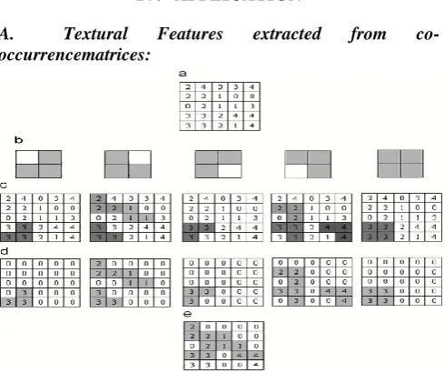
Figure. 5. The flow chart of textons detecting: (a) original image, (b) five special types of textons, (c) textons detection (d) five components of texton

images and (e) the final texton image.

Our initial assumption in characterizing image texture is that all the texture information is contained in the gray-tone spatial-dependence matrices. Hence all the textural features we suggest are extracted from these gray-tone spatial-dependence matrices. Some of these measures relate to specific textural characteristics of the image such as homogeneity, contrast, and the presence of organized structure within the image. Other measures characterize the complexity and nature of gray tone transitions which occur in the image. Even though these features contain information about the textural characteristics of the image, it is hard to identify which specific textural characteristic is represented by each of these features.

B. Calculation of texton co-occurrence matrix:

Julesz proposed the term “texton” conceptually more than 20 years ago.[4,5] Texton is a very useful concept in texture analysis. As a general rule, texton defined as a set of blobs or emergent patterns sharing a common property all over the image; however, defining textons remains a challenge.

The image features have a close relationship with textons and color diversification. The difference of textons may form various image Features. If the textons in image are small and the tonal differences between neighboring textons are large, a fine texture may result. If the textons are larger and consist of several pixels, a coarse texture may result. At the same time,

the textons in image are large and consist of a coarse texture characteristic depends on scale. If the textons in image are large and consist of a few texton categories, an obvious shape may result few texton categories, an obvious shape may result.

There are many types of textons in images [6,9]. In this paper, we only define five special types of textons for image analysis. Let there is a 2×2 grid in image. Its pixels are V1,V2,V3and V4 if three or four pixel values special types of textons are denoted as are same, thus those pixels formed a texton. Those five T1,T2,T3,T4,and T5 It is shown in Fig. 4, the shadow of 2×2 grid denotes those pixel values are same. Different shadow structure formed various textonsis an image, if it is shifted by one pixel in every direction, a 2×2 grid may appear.

Figure. 4 Five special types of texto ns: (a) 2 ×2 grid; (b) T1; (c) T2;(d) T3;(e)T4;(f) and T5

We use those five special types of textons to detect every grid, respectively, and then find out whether one of them may appear in those grids. A type of texton may detect out a component of texton image, thus there are five components of texton images. It is shown in Fig5(c). In those five components of texton images, the pixels of textons are kept in original values, others are replaced with the value of 0. It is shown in Fig. 5(d). Finally, we will combine those five components of texton images together to form a final textons image. Let the pixel position is P = (X,Y) ), at the same position Pi = (x,y), every component of texton image has a pixel value, thus five components of texton images have five pixel values. They are denoted as W1,W2,W3,W4 and W5 If those five pixel values are same, the final texton image will be kept in original, values in corresponding positions. If the values of 0 and nonzero appear in those five pixels, the final textons image will be kept in the values of nonzero. It is shown in Fig. 5(e).

V. CONCLUSION

In this paper, we have put forward a new method of co occurrence matrix to describe image features. It is different from the gray co-occurrence matrix and color correlograms because this method has the discrimination power of shape features. Image retrieval experiments were conducted over two image database sets using the gray co-occurrence matrix, color correlograms and the texton co-occurrence matrix. The two image database sets mainly come from VisTex texture database of MIT, Corel images and web. Experimental results have shown that our proposed method has the discrimination power of color, texture and shape features, the performances are better than that of GLCM and CCG.

VI. REFERENCE

[1]. Guang-Hai Liu, Jing-Yu Yang., Image retrieval based on the texton co-occurrence matrix in IEEE Conference on Computer Vision and Pattern Recognition, 2009.

[3]. G. Cross, A. Jain, Markov random field texture models, IEEE Trans. Pattern Anal Mach. Intell. 5 (1) (1983) 25–39.

[4]. J. Mao, A. Jain, Texture classification and segmentation using multi-resolution simultaneous autoregressive models, Pattern Recognition 25 (2) (1992) 173–188.

[5]. F. Liu, R. Picard, Periodicity, directionality, and randomness: wold features for image modeling and retrieval, IEEE Trans. Pattern Anal. Mach. Intell. 18 (7) (1996) 722–733.

[6]. B.S. Manjunath, W.Y. Ma, Texture features for browsing and retrieval of image data, IEEE Trans. Pattern Anal. Mach. Intell. 18 (8) (1996) 837–842.

[7]. J. Han, K.-K. Ma, Rotation-invariant and scale-invariant Gabor features for texture image retrieval, Image Vision Comput. 25 (2007) 1474–1481.

[8]. T. Chang, C.C. Jay Kuo, Texture analysis and classification with tree-structured wavelet transform, IEEE Trans. Image Process. 2 (4) (1993) 429–441.

[9]. A. Laine, J. Fan, Texture classification by wavelet packet signatures, IEEE Trans. Pattern Anal. Mach. Intell. 11 (15) (1993) 1186–1191.

[10]. M. Sonka, V. Hlavac, R. Boyle, Image Processing, Analysis, and Machine Vision, second ed., Thomson Brooks/Cole, Boston, MA, USA, 1998.