Handling Missing Values in A Dataset

Volume 3, No. 5, Sept-Oct 2012

International Journal of Advanced Research in Computer Science

RESEARCH PAPER

Available Online at www.ijarcs.info

ISSN No. 0976-5697

Handling Missing Values in A Dataset

Emeka, Chinedu E*

Department of Computer Science Nnamdi Azikiwe University, Awka

Anambra State, Nigeria [email protected]

Okonkwo Obi R

Department of Computer Science Nnamdi Azikiwe University, Awka

Anambra State, Nigeria oobi2971@ yahoo.com

Abstract: In predictive data mining, all issues pertaining to missing values in a dataset must be resolved before modeling can commence. Careful analysis and planning is required in the process of filling missing values to avoid introduction of artificial patterns, which may erroneously be discovered during modeling. In this work, four techniques: “Replacement with mean”, “Replacement with nearest neighbor”, “Replacement with regression analysis” and “Discard columns with missing values” were used to fill missing values in “offences against persons” 1980 - 2008 dataset obtained from the Nigeria Police Force. The dataset was divided into two; test set 1980 - 2003 (containing the filled in values) and holdout sample for validation 2004 – 2008. The test data was used to predict the holdout sample data – the objective being to determine which technique predicted the best match to actual data. The “Discard columns with missing values” technique achieved a correlation coefficient of -0.45 in one run. This work has demonstrated that missing values in a dataset can be handled and need not abort the data mining process.

Keywords: data mining; missing values; data preparation; replacement; correlation

I. INTRODUCTION

The data mining process can be broadly divided into four stages. These stages are: (1) Problem Definition, (2) Data Gathering & Preparation, (3) Model Building & Evaluation and (4) Knowledge Deployment - see Fig. 1 below. Once the problem definition has been articulated by translating the real world situation into a more tangible and useful data mining problem statement, the data gathering and preparation stage commences. One of the main problems encountered during data gathering & preparation is how to deal with missing values. This issue is investigated in this work using the dataset “Offences against persons” (1980 – 2008) obtained from the Nigeria Police Force (NPF) [1][2][3].

Figure 1: The Data mining process

The NPF compiles crimes in categories of offences. One of these categories is offences against persons which comprises of: Murder, attempted murder, manslaughter, suicide, attempted suicide, grievous harm & wounding, assault, child stealing, slave dealing, rape & indecent assault, kidnapping, unnatural offences, other offences (related to crimes against persons). Table 1 below shows offences against persons from 1980 – 2008.

Table 1: Offences against persons

Ye a r M ur de r a tte m p te d m ur de r man sl au gh te r sui c ide a tte m p te d sui c ide g/ h ar m & w o und ing a ssa u lt c h ild st e a lin g sl ave de a li ng r a p e /in d ic e nt a ss a ul t ki d na p pi ng un na tur a l o ff en ce s o th er o ff en ce s

1980 1633 183 79 261 - 10571 37203 390 15 2361 - 170 3019

1981 1520 184 46 183 - 11559 39402 252 6 2079 - 356 8759

1982 1786 - 218 481 - 15507 55153 360 21 2805 - 398 1253

1983 1857 223 174 223 - 15758 52204 197 25 1775 - 425 18678

1984 1548 193 123 197 142 13439 49413 199 19 2647 265 328 17741

1986 1539 181 94 192 155 15965 50009 125 27 2763 281 812 48166

1987 1657 208 65 133 138 15445 49472 157 41 2248 330 806 -

1988 1688 195 51 700 106 15388 60775 240 41 2368 387 697 -

1989 1586 157 69 176 98 15851 51757 95 33 2032 361 1610 25037

1990 1587 157 69 126 102 16429 49291 204 56 2181 374 778 25004

1991 1502 174 53 164 111 14775 51312 174 28 2227 354 314 23228

1992 1452 228 48 156 135 16491 53320 230 13 2261 400 311 21715

1993 1684 304 44 182 87 16361 51918 97 42 2307 371 289 20086

1994 1629 259 20 200 291 17167 46924 131 33 2364 461 685 20114

1995 1585 321 25 229 120 16300 46543 175 16 2364 415 462 18227

1996 1561 307 21 238 77 17605 52747 146 7 2198 373 419 16922

1997 1730 250 18 272 58 14720 42815 303 17 2585 377 435 17355

1998 1670 248 27 313 43 14362 40764 107 11 2249 282 516 17009

1999 1645 220 14 323 30 15931 33881 147 21 2241 342 456 13467

2000 1255 76 101 146 41 9756 17909 101 11 1529 243 376 12097

2001 2120 253 14 241 27 15241 37531 116 45 2284 349 434 17349

2002 2117 267 13 152 29 17580 29329 55 17 2084 337 277 14475

2003 2136 233 6 191 38 17666 29125 39 18 2253 410 306 15037

2004 2550 315 23 131 19 18733 29863 45 18 1626 349 265 11600

2005 2074 283 11 128 20 22858 33991 80 14 1835 798 371 9333

2006 2000 389 2 199 51 26434 32838 59 11 1718 372 361 10151

2007 1981 328 11 154 43 6175 15136 65 5 1545 277 585 8523

2008 1956 261 17 141 21 6405 14692 64 10 1359 309 233 9647

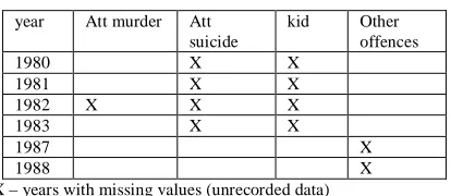
The Police dataset is characterized by unrecorded values in the following years:

Table 2: Breakdown of missing values

year Att murder Att suicide

kid Other offences

1980 X X

1981 X X

1982 X X X

1983 X X

1987 X

1988 X

Key : X – years with missing values (unrecorded data)

Unrecorded data can be broadly categorized into Missing and Empty values. Empty values have not been initialized and are not known. In other words, empty values have no corresponding real world values. On the other hand, missing values have corresponding real world values that were not captured during data collection. In data mining, it is important to resolve all issues pertaining to missing and empty values before data can be used for modeling. Handling of missing

values is an important aspect of data preparation. Often times, fields with missing values arise from not capturing the available data. For example, in 1982, 1786 cases of murder were recorded while no case of attempted murder was recorded. For this to be true, it means that every one who tried to murder somebody was successful 100% (all) of the time.

This clearly indicates that the value is not an “empty” value but a “missing” value. For this same reason, the unspecified values for attempted suicide from 1980 – 1983 can be assume to be missing values. “Other offences” is an aggregation of offences against persons not specifically suited for inclusion in any of the twelve defined categories. In 1986, 48166 “Other offences” were recorded and in 1989, 25037 “Other offences” were recorded. However, in 1987 and 1988, no “Other offences” were recorded. It is unlikely that the NPF prevented all “Other offences” in those two years but failed to do so in other years. Therefore, this is also a case of “missing” values. For the same reason, the unrecorded values for kidnapping (1980 – 1983) are regarded as “missing” values.

a. There may be some information content, predictive or inferential, carried by the actual pattern of measurements missing.

b. In creating and inserting some replacement values for missing values, care must be taken to insert values that neither adds nor subtracts information from the dataset.

The objective of this study is to propose a suitable technique that can be used to create and insert replacement values for missing values in a dataset bearing in mind the constraint placed by (b).

II. METHODOLOGY

The following techniques were used to derive values for the missing fields.

a. Replacement with mean: in this case, the mean of

the column with a missing field is used to replace any missing field in the column.

b. Replacement with nearest neighbor: in this case, the

value nearest to a missing field in the column with the missing field is used to replace the missing field. If preceding and succeeding values exist, the preceding value is selected.

c. Replacement with regression analysis: in this case, a

regression equation is derived for the dependent variable (column with a missing value). The regression equation is then used to compute a value for the missing field.

d. Discard columns with missing values: in this case,

any column with a missing value is discarded.

The correlation coefficient is a measurement of the strength of the linear relationship between two variables. The resulting values are always between -1 and +1. A result value near or equal to 0 implies little or no linear relationship between actual and predicted values. A value close to 1 indicates a strong positive linear relationship and a value close to -1 indicates a strong negative linear relationship. The formula for computing Correlation coefficient is:

Where ΣҮ = sum of the actual observed values, ΣΧ = sum

of the predicted values, ΣҮ 2

= sum of squares of the actual

observed values, ΣΧ2

= sum of squares of the predicted values,

ΣΧҮ = sum of each actual observed value multiplied by its

corresponding predicted value and n is the number of observations. The correlation coefficient is suitable to determine the best replacement technique i.e. the technique that produces the highest correlation coefficient will be adjudged the best for filling missing values in the dataset used in this study.

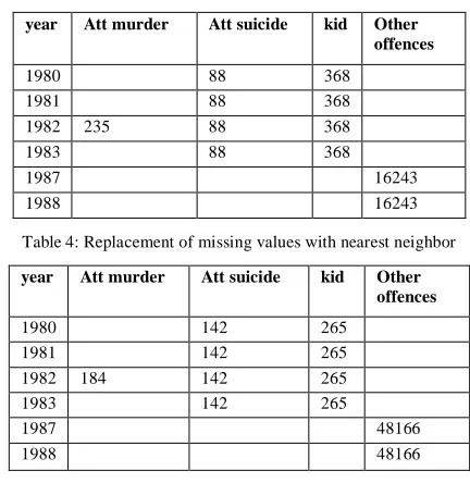
Tables 3 and 4 shows the values derived for the missing fields using “replacement with mean” and “replacement with nearest neighbor” respectively.

Table 3: Replacement of missing values with mean

year Att murder Att suicide kid Other offences

1980 88 368

1981 88 368

1982 235 88 368

1983 88 368

1987 16243

1988 16243

Table 4: Replacement of missing values with nearest neighbor

year Att murder Att suicide kid Other offences

1980 142 265

1981 142 265

1982 184 142 265

1983 142 265

1987 48166

1988 48166

Regression analysis is used to investigate relationships between variables. In simple linearregression, there is a single independent variable (X) and a single dependent variable (Y). Multiple linear regression is an extension of simple linear regression in which more than one independent variable (X) is used to predict a single dependent variable (Y). To generate a multiple linear regression model, estimates for the coefficients are derived from the training data. The objective of the process is to identify the best fitting model for the data. All the independent variables play a role in determining the dependent variable therefore an expert with knowledge of the subject matter is required to determine variables relevant to the analysis at hand. In this case, it is assumed that all the variables in “offences against persons” are relevant.

The regression equations are:

attempted murder = 122.039 + 0.086Murder + -0.723manslaughter + -0.034suicide + 0.001g/harm &

wounding + 0.003assault + -0.095child stealing + -0.805slave dealing + -0.028rape/indicent assault + -0.049unnatural offences

attempted suicide = 99.564 + 0.085Murder +

-0.101manslaughter + -0.105suicide + 0g/harm & wounding + 0.001assault + -0.062child stealing + 1.017slave dealing + 0.045rape/indicent assault + 0.011unnatural offences

kidnapping = 285.161 + -0.003Murder + -1.034manslaughter + -0.128suicide + 0.013g/harm & wounding + 0assault + 0.394child stealing + 0.576slave dealing + -0.065rape/indicent assault + 0.011unnatural offences

other offences = 1788.399 + -3.67Murder +

-27.956slave dealing + 14.514rape/indicent assault + 6.771unnatural offences.

The correlation coefficients are:

Table 5: Correlation coefficients of derived equations

Variable Correlation coefficient

Attempted murder 0.8074652

Attempted suicide 0.7402702

Kidnapping 0.6542171

Other offences 0.8485281

Solving the equations yielded the results in table 6 below.

Table 6: Replacement of missing values with regression analysis

year Att murder Att suicide kid Other offences

1980 62 313

1981 74 331

1982 133 60 170

1983 51 257

1987 26316

1988 -5139

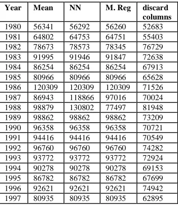
After replacement of missing values with values derived from each technique, the figures were summed to obtain summary of “offences against persons” for each technique. Table 7 shows “offences against persons” derived from each technique – note that for “replacement with mean”, “replacement with nearest neighbor” (NN) and “replacement with regression analysis” (M, Reg), all figures are the same except for 1980 – 1983 and 1987 – 1988 (the years with missing fields). Note also that because “attempted murder”, “attempted suicide”, “kidnapping” and “other offences” (columns with missing fields) have been removed in “Discard columns with missing values”, all values in “Discard columns with missing values” are lower than actual recorded values.

Table 7: Summary of offences against persons

Year Mean NN M. Reg discard columns 1980 56341 56292 56260 52683 1981 64802 64753 64751 55403 1982 78673 78573 78345 76729 1983 91995 91946 91847 72638 1984 86254 86254 86254 67913 1985 80966 80966 80966 65628 1986 120309 120309 120309 71526 1987 86943 118866 97016 70024 1988 98879 130802 77497 81948 1989 98862 98862 98862 73209 1990 96358 96358 96358 70721 1991 94416 94416 94416 70549 1992 96760 96760 96760 74282 1993 93772 93772 93772 72924 1994 90278 90278 90278 69153 1995 86782 86782 86782 67699 1996 92621 92621 92621 74942 1997 80935 80935 80935 62895

1998 77601 77601 77601 60019 1999 68718 68718 68718 54659 2000 43641 43641 43641 31184 2001 76004 76004 76004 58026 2002 66732 66732 66732 51624 2003 67458 67458 67458 51740 2004 65537 65537 65537 53254 2005 71796 71796 71796 61362 2006 74585 74585 74585 63622 2007 34828 34828 34828 25657 2008 35115 35115 35115 24877

Figure 2 below is a 3D plot of the dataset produced by each technique.

0 20000 40000 60000 80000 100000 120000 140000

1 2 3 4 5 6 _{7 8 9 10 11}

12 13 14 15 16_{17 18 19 20}

21 22 23 24_{25 26 27 28} 29 offences against persons

Mean nearest neighbor multiple regression discard columns

Figure 2: Offences against persons with missing values replaced

III. EXPERIMENTATION

Neural networks are suitable for prediction, forecasting, categorization and classification problems [5]. A Multi Layer Perceptron (MLP) is a feed forward neural network with one or more hidden layers. One of the main learning tasks for the multilayer perceptron is function regression. The function regression task can be regarded as the problem of approximating a function from an input-target dataset [6]. The targets are a specification of what the output response to the inputs should be. Learning proceeds by presenting an input pattern to the network. The network then propagates the input pattern from layer to layer until the output pattern is generated by the output layer. If this pattern is different from the desired output, an error is calculated and then propagated backwards through the network from the output layer to the input layer.

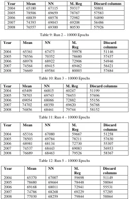
each technique are displayed in tables 8,9,10,11, and 12 below:

Table 8: Run 1 – 10000 Epochs

Year Mean NN M. Reg Discard columns 2004 65180 67115 59317 50801

2005 78506 69659 78767 57583 2006 68839 68578 72982 54890 2007 74393 69043 69208 56486 2008 76557 69300 80530 57926

Table 9: Run 2 – 10000 Epochs

Year Mean NN M. Reg

Discard columns 2004 65361 67473 59978 51146 2005 78556 70352 78680 57437 2006 68978 68922 72906 54946 2007 74564 69415 69462 56421 2008 76669 69584 80003 57684

Table 10: Run 3 – 10000 Epochs

Year Mean NN M. Reg Discard columns 2004 65409 66815 60247 51199

2005 78703 69743 78453 57696 2006 69054 68066 72882 55156 2007 74702 68350 69620 56768 2008 76856 68461 79744 58152

Table 11: Run 4 – 10000 Epochs

Year Mean NN M. Reg

Discard columns 2004 65316 67080 59667 51258 2005 78503 69784 78211 57630 2006 68981 68134 72730 55307 2007 74537 68443 69083 56953 2008 76689 68463 79526 58367

Table 12: Run 5 – 10000 Epochs

Year Mean NN M. Reg

Discard columns 2004 65370 67007 59698 51149 2005 78680 69664 78448 58064 2006 69168 68011 72941 55531 2007 74786 68268 69229 57285 2008 77030 68259 79844 58864

Validation was carried out by computing the correlation coefficient of each run. In this case, the variables are the actual values of “offences against persons” 2004 – 2008 (table 13 below) and predicted values of “offences against persons” 2004 – 2008 (tables 8,9,10,11 and 12).

Table 13: offences against persons 2004 - 2008

Year Offences against persons

2004 65537

2005 71796

2006 74585

2007 34828

2008 35115

Table 14 below is the summary of correlation coefficients.

Table 14: Summary of Correlation coefficients

Run Mean NN M. Reg

Discard columns 1 -0.3828 -0.2818 -0.1712 -0.4128 2 -0.3881 -0.1879 -0.1659 -0.4075 3 -0.3909 -0.0013 -0.1697 -0.4285 4 -0.3902 0.0279 -0.1593 -0.4535 5 -0.3985 0.0729 -0.1606 -0.4510

IV. ANALYSIS

As stated earlier, the values in “Discard columns with missing values” dataset are different (lower in all cases) from the actual observed values in the Police dataset. Therefore, any analysis involving this dataset is unrelated and irrelevant to “offences against persons”. The higher than others correlation coefficient achieved by this technique (-0.4535 in run 4) must be disregarded. The fact that most values in the holdout sample data are low made “Discard columns with missing values” to produce a spuriously good correlation coefficient. The “Replacement with nearest neighbor” technique produced instances of positive and negative correlation i.e., run 1 – 3 produced negative correlations while run 4 and 5 produced positive correlations. Besides the fact that the correlation coefficients are low (-0.2818 in run 1), the shift from negative to positive correlation implies that the technique is unstable and predictions made (with this dataset) cannot be relied upon. The “Replacement with mean” technique produced correlation coefficients ranging from -0.383 (run 1) to -0.399 (run 5). Though this cannot be considered to be an indication of a strong negative correlation, it was consistent in five runs. The maximum variation it produced in correlation coefficients calculated for the five runs was 0.016.

The “Replacement with regression analysis” technique yielded a low correlation ranging from -0.159 (run 4) to -0.171 (run 1). But like the “Replacement of missing values with mean” technique, it was consistent in that all runs produced a negative correlation. Table 5 shows the correlation coefficients of the equations produced by “Replacement of missing values with regression analysis”. These correlation coefficients can be increased by deriving equations that more aptly fit the dataset. Non linear regression can be used to derive such equations.

V. CONCLUSION

This work has shown that when missing values are encountered in a dataset, the values can be handled (filled) and that the data mining process need not be aborted. It has also shown that “Replacement of missing values with mean” and “Replacement of missing values with regression analysis” can be used to fill missing values in a dataset.

VI. REFERENCES

[2]. The Annual Abstract of Statistics (1980 - 2009). Published by The NATIONAL BUREAU OF STATISTICS , Abuja, Nigeria

[3]. CLEEN FOUNDATION – Nigeria (2009). official crime statistics. http://www.cleen.org/officialcrimestatistic.html (Retrieved February, 2010)

[4]. Pyle, D. (1999). Data preparation for data mining Morgan Kaufmann Publishers, USA pp. 275 – 297

[5]. Swingler, K., (1996). Applying neural networks; a practical guide. San Francisco; Morgan Kaufman

[6]. Bishop, C., (1995). Neural Networks for Pattern Recognition. Oxford University Press.