How to Solve Classification and Regression Problems on
High-Dimensional Data with a Supervised
Extension of Slow Feature Analysis
Alberto N. Escalante-B. [email protected]
Laurenz Wiskott [email protected]
Theory of Neural Systems Institut f¨ur Neuroinformatik Ruhr-University of Bochum Bochum D-44801, Germany
Abstract
Supervised learning from high-dimensional data, e.g., multimedia data, is a challenging task. We propose an extension of slow feature analysis (SFA) forsuperviseddimensionality reduction called graph-based SFA (GSFA). The algorithm extracts a label-predictive low-dimensional set of features that can be post-processed by typical supervised algorithms to generate the final label or class estimation. GSFA is trained with a so-called training graph, in which the vertices are the samples and the edges represent similarities of the corresponding labels. A new weighted SFA optimization problem is introduced, generalizing the notion of slowness from sequences of samples to such training graphs. We show that GSFA computes an optimal solution to this problem in the considered function space, and propose several types of training graphs. For classification, the most straightforward graph yields features equivalent to those of (nonlinear) Fisher discriminant analysis. Emphasis is on regression, where four different graphs were evaluated experimentally with a subproblem of face detection on photographs. The method proposed is promising particularly when linear models are insufficient, as well as when feature selection is difficult.
Keywords: Slow feature analysis, feature extraction, classification, regression, pattern recognition, training graphs, nonlinear, dimensionality reduction, supervised learning, high-dimensional data, implicitly supervised, image analysis.
1. Introduction
This limits the practical applicability of supervised learning, frequently resulting in lower performance and higher computational requirements.
Unsupervised dimensionality reduction, including algorithms such as PCA or LPP (He and Niyogi, 2003), can be used to attenuate these problems. After dimensionality reduction, typical supervised learning algorithms can be applied. Frequent benefits include a lower computational cost and better robustness against overfitting. However, since the final goal is to solve a supervised learning problem, this approach is inherently limited.
Supervised dimensionality reduction is more appropriate in this case. Its goal is to compute a low-dimensional set of features from the high-dimensional input samples that contains predictive information about the labels (Rish et al., 2008). One advantage is that dimensions irrelevant for the label estimation can be discarded, resulting in a more com-pact representation and more accurate label estimations. Different supervised algorithms can then be applied to the low-dimensional data. A widely known algorithm for supervised dimensionality reduction is Fisher discriminant analysis (FDA) (Fisher, 1936). Sugiyama (2006) proposed local FDA (LFDA), an adaptation of FDA with a discriminative objec-tive function that also preserves the local structure of the input data. Later, Sugiyama et al. (2010) proposed semi-supervised LFDA (SELF) bridging LFDA and PCA, and al-lowing the combination of labeled and unlabeled data. Tang and Zhong (2007) introduced pairwise constraints-guided feature projection (PCGFP), where two types of constraints are allowed. Must-link constraints denote that a pair of samples should be mapped closely in the low-dimensional space, while cannot-link constraints require that the samples are mapped far apart. Later, Zhang et al. (2007) proposed semi-supervised dimensionality reduction (SSDR), which is similar to PCGFP and also supports semi-supervised learning.
SFA has been used to solve regression problems as well. Franzius et al. (2008) used stan-dard SFA to learn the position of animated fish from images with homogeneous background. In this particular setup, the position of the fish was changed at a relatively slow pace. SFA was thus trained in a completely unsupervised way. A number of extracted slow features were then post-processed with linear regression (coupled with a nonlinear transformation). In this article, we introduce a supervised extension of SFA called graph-based SFA (GSFA) specifically designed for supervised dimensionality reduction. We show that GSFA computes the slowest features possible according to a generalized concept of signal slowness formalized by a weighted SFA optimization problem described below.
The objective function of this optimization problem is a weighted sum of squared output differences, and is therefore similar to the underlying objective functions of, for example, FDA, LFDA, SELF, PCGFP, and SSDR. However, in general the optimization problem solved by GSFA differs at least in one of the following elements: a) the concrete coefficients of the objective function, b) the constraints, or c) the feature space considered. Although kernelized versions of the algorithms above can be defined, one has to overcome the difficulty of finding a good kernel. In contrast, SFA (and GSFA) was conceived from the beginning as a nonlinear algorithm without resorting to kernels, with linear SFA being just a less used special case. Another difference with various algorithms above is that SFA (and GSFA) does not explicitly attempt to preserve the structure of the data. Interestingly, features equivalent to those of FDA can be obtained if particular training data is given to GSFA.
There is a close relation between SFA and Laplacian eigenmaps (LE), which has been studied by Sprekeler (2011). GSFA and LE have the same objective function, but in gen-eral GSFA uses different edge-weight (adjacency) matrices, has different normalization con-straints, supports node-weights, and uses function spaces.
One advantage of GSFA is that it is designed for classification and regression, while most algorithms for supervised dimensionality reduction, including the ones above, focus on classification only.
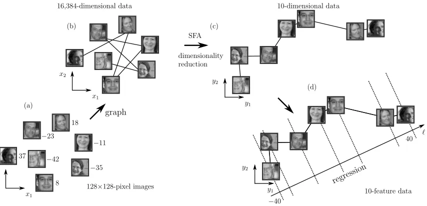
The central idea behind GSFA is to encode the label information implicitly in the struc-ture of the input data, as some type of similarity matrix called edge-weight matrix, to indirectly solve the supervised learning problem, rather than performing an explicit fit to the labels. The full input data, called training graph, then takes the form of a weighted graph with vertices representing the data points (samples), node weights specifying a pri-orisample probabilities, and edge weights indicating desired output similarities, as derived from the labels. Details are given in Section 3. This permits us to extend SFA to extract features from the data points that tend to reflect similarity relationships between their la-bels without the need to reproduce the lala-bels themselves. An illustration of the method is provided in Figure 1. This has several advantages that originate from SFA:
• SFA has a complexity ofO(N) in the number of samplesN and O(I3) in the number of dimensionsI (possibly after a nonlinear expansion). Hierarchical processing greatly reduces the later complexity down toO(IlogI). In practice, processing 100,000 sam-ples of 10,000-dimensional input data can be done in less than three hours by using hierarchical SFA without resorting to parallelization or GPU computing.
• The SFA algorithm itself is almost parameter free. Only the nonlinear expansion has to be defined. In hierarchical SFA, the structure of the network has several parameters, but the choice is usually not critical. Typically no expensive parameter search is required.
Figure 1: Illustration of the use of GSFA to solve a regression problem. An input sample is an image represented as a 16384-dimensional vector,x, and yields a 2-dimensional feature vector y. (a) Original images and their labels indicating the horizontal position of the face center. (b) A graph with appropriate pairwise connections between the samples is created. Here only images with most similar labels are connected resulting in a linear graph. (c) Example of the low-dimensional GSFA output. Notice how the first slow component,y1, is strongly related to the original label. (d) The result of regression, thus, ideally depends only ony1.
regression problem closely related to face detection using real photographs. A discussion section concludes the article.
2. Standard SFA
2.1 The slowness principle and SFA
Perception plays a crucial role in the interaction of animals or humans with their environ-ment. Although processing of sensory information appears to be done straightforwardly by the nervous system, it is a complex computational task. As an example, consider the visual perception of a driver watching pedestrians walking on the street. As the car advances, his receptor responses typically change quite quickly, and are especially sensitive to the eye movement, and to variations in the position or pose of the pedestrians. However, a lot of information, including the position and identity of the pedestrians, can still be dis-tinguished. Relevant abstract information derived from the perception of the environment typically changes on a time scale much slower than the individual sensory inputs. This observation inspires the slowness principle, which explicitly requires the extraction of slow features. This principle has probably first been formulated by Hinton (1989), and online learning rules were developed shortly after by F¨oldi´ak (1991) and Mitchison (1991). The first closed-form algorithm has been developed by Wiskott and is referred to as Slow feature analysis (SFA, Wiskott, 1998; Wiskott and Sejnowski, 2002). The concise formulation of the SFA optimization problem also permits an extended mathematical treatment so that its properties are well understood analytically (Wiskott, 2003; Franzius et al., 2007; Sprekeler and Wiskott, 2011). SFA has the advantage that it is guaranteed to find an optimal solution within the considered function space. It was initially developed for learning invariances in a model of the primate visual system (Wiskott and Sejnowski, 2002; Franzius et al., 2011). Berkes and Wiskott (2005) subsequently used it for learning complex-cell receptive fields and Franzius et al. (2007) for place cells in the hippocampus. Recently, researchers have begun using SFA for various technical applications (Escalante-B. and Wiskott, 2012).
2.2 Standard SFA optimization problem
The SFA optimization problem can be stated as follows (Wiskott, 1998; Wiskott and Se-jnowski, 2002; Berkes and Wiskott, 2005). Given an I-dimensional input signal x(t) = (x1(t), . . . , xI(t))T, where t∈R, find an instantaneous vectorial function g:RI →RJ, i.e., g(x(t)) = (g1(x(t)), . . . , gJ(x(t)))T, within a function spaceFsuch that for each component
yj(t) def
= gj(x(t)) of the output signaly(t) def
= g(x(t)), for 1≤j ≤J, the objective function
∆(yj) def
= hy˙j(t)2itis minimal (delta value) (1)
under the constraints
hyj(t)it= 0 (zero mean), (2)
hyj(t)2it= 1 (unit variance), (3)
The delta value ∆(yj) is defined as the time average (h·it) of the squared derivative
of yj and is therefore a measure of the slowness (or rather fastness) of the signal. The
constraints (2–4) assure that the output signals are normalized, not constant, and represent different features of the input signal. The problem can be solved iteratively beginning with
y1 (the slowest feature extracted) and finishing with yJ (an algorithm is described in the
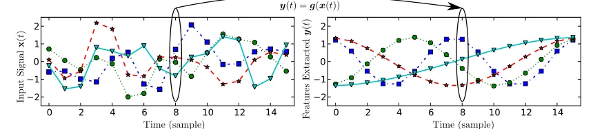
next subsection). Due to constraint (4), the delta values are ordered, i.e., ∆(y1)≤∆(y2)≤ · · · ≤∆(yJ). See Figure 2 for an illustrative example.
0 2 4 6 8 10 12 14
2 1 0 1 2
Figure 2: Illustrative example of feature extraction from a 10-dimensional (discrete time) input signal. Four arbitrary components of the input (left) and the four slowest outputs (right) are shown. Notice that feature extraction is an instantaneous operation, even though the outputs are slow over time. This example was designed such that the features extracted are the slowest ones theoretically possible.
In practice, the function g is usually restricted to a finite-dimensional spaceF, e.g., to all quadratic or linear functions. In theoretical analyses (e.g., Wiskott, 2003) it is common to use an unrestricted function space.
2.3 Standard linear SFA algorithm
The SFA algorithm is typically nonlinear. Even though a kernelized version has been pro-posed (Bray and Martinez, 2003; Vollgraf and Obermayer, 2006), it is usually implemented more directly with a nonlinear expansion of the input data followed by linear SFA in the expanded space. In this section, we recall the standard linear SFA algorithm (Wiskott and Sejnowski, 2002), in which F is the space of all linear functions. Discrete time, t ∈ N, is used for the application of the algorithm to real data. Also the objective function and the constraints are adapted to discrete time. The input is then a single training signal (i.e., a sequence of N samples) x(t), where 1 ≤t ≤N, and the time derivative of x(t) is usually
approximated by a sequence of differences of consecutive samples: ˙x(t)def≈ x(t+ 1)−x(t), for 1≤t≤N−1.
The output components take the form gj(x) = wjT(x−x¯), where ¯x def
= N1 PN
t=1x(t)
The covariance matrix h(x−µx)(x−µx)Tit is approximated by the sample covariance
matrix
C= 1
N −1
N
X
t=1
(x(t)−x¯)(x(t)−¯x)T , (5)
and the derivative second-moment matrixhx˙x˙Tit is approximated as
˙
C= 1
N−1
N−1
X
t=1
(x(t+ 1)−x(t))(x(t+ 1)−x(t))T. (6)
Then, a sphered signalzdef= STxis computed, such thatSTCS=Ifor a sphering matrix S. Afterwards, the J directions of least variance in the derivative signal ˙z are found and represented by anI×J rotation matrixR, such thatRTCzR˙ =Λ, whereCz˙ def= h˙z ˙zTitand Λ is a diagonal matrix with diagonal elements λ1 ≤λ2 ≤ · · · ≤ λJ. Finally the algorithm
returns the weight matrix W = (w1, . . . ,wJ), defined as W =SR, the features extracted y=WT(x−x¯), and ∆(yj), for 1≤j ≤J. The linear SFA algorithm is guaranteed to find
an optimal solution to the optimization problem in the linear function space (Wiskott and Sejnowski, 2002), e.g., the first component extracted is the slowest possible linear feature.
The complexity of the linear SFA algorithm described above is O(N I2 +I3) where
N is the number of samples and I is the input dimensionality (possibly after a nonlinear expansion), thus for high-dimensional data standard SFA is not feasible1. In practice, it has a speed comparable to PCA, even though SFA also takes into account the temporal structure of the data.
2.4 Hierarchical SFA
To reduce the complexity of SFA, a divide-and-conquer strategy to extract slow features is usually effective (e.g., Franzius et al., 2011). For instance, one can spatially divide the data into lower-dimensional blocks of dimension I0 I and extract J0 < I0 local slow features separately with different instances of SFA, the so-called SFA nodes. Then, one uses another SFA node in a next layer to extract global slow features from the local slow features. Since each SFA node performs dimensionality reduction, the input dimension of the top SFA node is much less thanI. This strategy can be repeated iteratively until the input dimensionality at each node is small enough, resulting in a multi-layer hierarchical network. Due to information loss before the top node, this does not guarantee optimal global slow features anymore. However it has shown to be effective in many practical experiments, in part because low-level features are spatially localized in most real data.
Interestingly, hierarchical processing can also be seen as a regularization method because the number of parameters to be learned is typically smaller than if a single SFA node with a huge input is used, leading to better generalization. An additional advantage is that the nonlinearity accumulates across layers, so that even when using simple expansions the network as a whole can realize a complex nonlinearity (Escalante-B. and Wiskott, 2011).
3. Graph-Based SFA (GSFA)
3.1 Organization of the training samples in a graph
Learning from a single (multi-dimensional) time series (i.e., a sequence of samples), as in standard SFA, is motivated from biology, because the input data is assumed to originate from sensory perception. In a more technical and supervised learning setting, the training data need not be a time series but may be a set of independent samples. However, one can use the labels to induce structure. For instance, face images may come from different persons and different sources but can still be ordered by, say, age. If one arranges these images in a sequence of increasing age, they would form a linear structure that could be used for training much like a regular time series.
The central contribution of this work is the consideration of a more complex structure for training SFA called training graph. In the example above, one can then introduce a weighted edge between any pair of face images according to some similarity measure based on age (or other criteria such as gender, race, or mimic expression), with high similarity resulting in large edge weights. The original SFA objective then needs to be adapted such that samples connected by large edge weights yield similar output values.
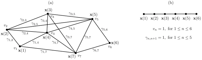
In mathematical terms, the training data is represented as a training graphG= (V,E) (illustrated in Figure 3) with a set V of vertices x(n) (each vertex/node being a sample), and a set E of edges (x(n),x(n0)), which are pairs of samples, with 1 ≤ n, n0 ≤ N. The indexn(orn0) substitutes the time variablet. The edges are undirected and have symmetric weights
γn,n0 = γn0,n (7)
that indicate the similarity between the connected vertices; also each vertex x(n) has an associated weight vn >0, which can be used to reflect its importance, frequency, or
relia-bility. For instance, a sample occurring frequently in an observed phenomenon should have a larger weight than a rare sample. This representation includes the standard time series as a special case in which the graph has a linear structure and all node and edge weights are identical (Figure 3.b). How exactly edge weights are derived from label values will be elaborated later on.
3.2 Weighted SFA optimization problem
We extend the concept of slowness, originally conceived for sequences of samples, to data structured in a training graph making use of its associated edge weights. The generalized optimization problem can then be formalized as follows. For 1≤j ≤J, find featuresyj(n),
where 1≤n≤N, such that the objective function
∆j def=
1
R
X
n,n0
γn,n0(yj(n0)−yj(n))2 is minimal (weighted delta value) (8)
under the constraints
1
Q
X
n
vnyj(n) = 0 (weighted zero mean), (9)
1
Q
X
n
vn(yj(n))2 = 1 (weighted unit variance), and (10)
1
Q
X
n
vnyj(n)yj0(n) = 0, forj0 < j (weighted decorrelation), (11)
with
Rdef= X
n,n0
γn,n0, (12)
Qdef= X
n
vn. (13)
Compared to the original SFA problem, the vertex weights generalize the normalization constraints, whereas the edge weights extend the objective function to penalize the difference between the outputs of arbitrary pairs of samples. Of course, the factor 1/Rin the objective function is not essential for the minimization problem, but it is useful for normalization purposes. Likewise, the factor 1/Qcan be dropped from (9) and (11).
By definition (see Section 3.1), training graphs are undirected, and have symmetric edge weights. This does not cause any loss of generality and is justified by the weighted optimization problem above. Its objective function (8) is insensitive to the direction of an edge because the sign of the output difference cancels out during the computation of ∆j. It
therefore makes no difference whether we chooseγn,n0 = 2 andγn0,n = 0 orγn,n0 =γn0,n = 1, for instance. We note also that γn,n multiplies with zero in (8) and only enters into the
calculation ofR. The variablesγn,n are kept only for mathematical convenience.
3.3 Linear graph-based SFA algorithm (linear GSFA)
Similarly to the standard linear SFA algorithm, which solves the standard SFA problem in the linear function space, here we propose an extension that computes an optimal solution to the weighted SFA problem within the same space. Let the verticesV={x(1), . . . ,x(N)}be the input samples with weights{v1, . . . , vN}and the edgesEbe the set of edges (x(n),x(n0))
version only in the computation of the matricesCand C˙, which now take into account the neighbourhood structure (samples, edges, and weights) specified by the training graph.
The sample covariance matrix CGis defined as:
CGdef= 1
Q
X
n
vn(x(n)−xˆ)(x(n)−xˆ)T =
1
Q
X
n
vnx(n)(x(n))T−xˆ(ˆx)T , (14)
where
ˆ
x def= 1
Q
X
n
vnx(n) (15)
is the weighted average of all samples. The derivative second-moment matrixC˙Gis defined as:
˙ CGdef=
1
R
X
n,n0
γn,n0 x(n0)−x(n) x(n0)−x(n)T. (16)
Given these matrices, the computation of W is the same as in the standard algorithm (Section 2.3). Thus, a sphering matrixS and a rotation matrix Rare computed with
STCGS = I, and (17)
RTSTC˙GSR = Λ, (18)
where Λ is a diagonal matrix with diagonal elements λ1 ≤ λ2 ≤ · · · ≤ λJ. Finally the
algorithm returns ∆(y1), . . . ,∆(yJ),W and y(n), where
W = SR, and (19)
y(n) = WT(x(n)−xˆ). (20)
3.4 Correctness of the graph-based SFA algorithm
We now prove that the GSFA algorithm indeed solves the optimization problem (8–11). This proof is similar to the optimality proof of the standard SFA algorithm (Wiskott and Sejnowski, 2002). For simplicity, assume that CG and C˙G have full rank.
The weighted zero mean constraint (9) holds trivially for anyW, because
X
n
vny(n) (20)= X
n
vnWT(x(n)−xˆ) (21)
= WT X
n
vnx(n)−X n0
vn0xˆ
!
(22)
(15,13)
We also find
I = RTIR (since Ris a rotation matrix), (24)
(17)
= RT(STCGS)R, (25)
(19)
= WTCGW, (26)
(14)
= WT 1 Q
X
n
vn(x(n)−xˆ)(x(n)−xˆ)TW, (27)
(20)
= 1
Q
X
n
vny(n)(y(n))T, (28)
which is equivalent to the normalization constraints (10) and (11). Now, let us consider the objective function
∆j (8)
= 1
R
X
n,n0
γn,n0 yj(n0)−yj(n)2 (29)
(16)
= wTjC˙Gwj (30)
(19)
= rTjSTC˙GSrj (31)
(18)
= λj, (32)
whereR= (r1, . . . ,rJ). The algorithm finds a rotation matrix Rsolving (18) and yielding
increasing λs. It can be seen (c.f. Adali and Haykin, 2010, Section 4.2.3) that this R also achieves the minimization of ∆j, forj = 1, . . . , J, hence, fulfilling (8).
3.5 Probabilistic interpretation of training graphs
In this section, we give an intuition for the relationship between GSFA and standard SFA. Readers less interested in this theoretical excursion can safely skip it. Given a training graph, we construct below a Markov chain M for the generation of input data such that the application of standard SFA to the input data yields the same features as GSFA does for the graph.
In order for this equivalence to hold, the vertex weights ˜vn and edge weights ˜γn,n0 of the graph must fulfil the following normalization restrictions:
X
n
˜
vn = 1, (33)
X
n0 ˜
γn,n0/˜vn = 1 ∀n , (34)
(7)
⇐⇒ X
n0 ˜
γn0,n/˜vn = 1 ∀n , (35)
X
n,n0 ˜
γn,n0
(34,33)
Restrictions (33) and (36) can be assumed without loss of generality, because they can be achieved by a constant scaling of the weights (i.e., ˜vn ← ˜vn/Q, ˜γn,n0 ← ˜γn,n0/R) without affecting the outputs generated by GSFA. The fundamental restriction is (34), which indi-cates (after multiplying with ˜vn) that each vertex weight should be equal to the sum of the
weights of all edges originating from such a vertex.
The Markov chain is then a sequence Z1,Z2,Z3, . . . of random variables that can
as-sume states that correspond to different input samples. Z1 is drawn from the stationary
distribution
π = p1 def= Pr(Z1 =x(n)) def= ˜vn, (37)
and the transition probabilities are given by
Pnn0 def= Pr(Zt+1 =x(n0)|Zt=x(n)) def= (1−)˜γn,n0/˜vn+˜vn0 =
lim→0
˜
γn,n0/v˜n, (38)
(37)
=⇒ Pr(Zt+1=x(n0),Zt=x(n)) = (1−)˜γn,n0+v˜n˜vn0 =
lim→0
˜
γn,n0, (39)
(for Zt stationary) with 0< 1. Due to the -term all states of the Markov chain can
transition to all other states including themselves, which makes the Markov chain irreducible and aperiodic, and therefore ergodic. Thus, the stationary distribution is unique and the Markov chain converges to it. The normalization restrictions (33), (34), and (36) ensure the normalization of (37), (38), and (39), respectively.
It is easy to see thatπ = ˜vn is indeed a stationary distribution, since for pt= ˜vn
pt+1 = Pr(Zt+1=x(n)) =
X
n0
Pr(Zt+1=x(n)|Zt=x(n0)) Pr(Zt=x(n0)) (40)
(37,38)
= X
n0
(1−) ˜γn0,n/v˜n0+v˜n˜vn0 (41)
(35,33)
= (1−)˜vn+v˜n = ˜vn = pt. (42)
The time average of the input sequence is
µZ def= hZtit (43)
= hZiπ (since Mis ergodic) (44)
(42)
= X
n
˜
vnx(n) (45)
(15)
= ˆx, (46)
and the covariance matrix is
C def= h(Z−µZ)(Z−µZ)Tit (47)
(46)
= h(Z−xˆ)(Z−xˆ)Tiπ (sinceMis ergodic) (48)
(42)
= X
n
˜
vn(x(n)−ˆx)(x(n)−xˆ)T (49)
(14)
whereas the derivative covariance matrix is
˙
C def= hZt˙ Z˙Ttit (51)
= hZ ˙˙ZTiπ (sinceMis ergodic) (52)
(39)
= X
n,n0
(1−)˜γn,n0+v˜nv˜n0(x(n0)−x(n))(x(n0)−x(n))T, (53)
whereZ˙t def
= Zt+1−Zt. Notice that lim→0C˙ (53)
= ˜γn,n0(x(n0)−x(n))(x(n0)−x(n))T (16)= C˙G. Therefore, if a graph fulfils the normalization restrictions (33)–(36), GSFA yields the same features as standard SFA on the sequence generated by the Markov chain, in the limit→0.
3.6 Construction of training graphs
One can, in principle, construct training graphs with arbitrary connections and weights. However, when the goal is to solve a supervised learning task, the graph created should implicitly integrate the label information. An appropriate structure of the training graphs depends on whether the goal is classification or regression. In the next sections, we describe each case separately. We have previously implemented the proposed training graphs, and we have tested and verified their usefulness on real-world data (Escalante-B. and Wiskott, 2010; Mohamed and Mahdi, 2010; Stallkamp et al., 2011; Escalante-B. and Wiskott, 2012).
4. Classification with SFA
In this section, we show how to use GSFA to profit from the label information and solve classification tasks more efficiently and accurately than with standard SFA.
4.1 Clustered training graph
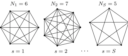
To generate features useful for classification, we propose the use of aclustered training graph
presented below (Figure 4). Assume there areS identities/classes, and for each particular identity s = 1, . . . , S there are Ns samples xs(n), where n = 1, . . . , Ns, making a total
of N = P
sNs samples. We define the clustered training graph as a graph G = (V,E)
with vertices V = {xs(n)}, and edges E = {(xs(n),xs(n0))} fors = 1, . . . , S, and n, n0 = 1, . . . , Ns. Thus all pairs of samples of the same identity are connected, while samples
of different identity are not connected. Node weights are identical and equal to one, i.e.,
∀s, n : vns = 1. In contrast, edge weights, γn,ns 0 = 1/Ns ∀n, n0, depend on the cluster
size2. Otherwise identities with a largeNs would be over-represented because the number
of edges in the complete subgraph for identitysgrows quadratically withNs. These weights
fulfil the normalization restriction (34). The optimization problem associated to this graph explicitly demands that samples from the same object identity should be typically mapped to similar outputs.
Figure 4: Illustration of a clustered training graph used for a classification problem. All samples belonging to the same object identity form fully connected subgraphs. Thus, forS identities there are S complete subgraphs. Self-loops not shown.
4.2 Efficient learning using the clustered training graph
At first sight, the large number of edges,P
sNs(Ns+ 1)/2, seems to introduce a
computa-tional burden. Here we show that this is not the case if one exploits the symmetry of the clustered training graph. From (14), the sample covariance matrix of this graph using the node weights vsn= 1 is (notice the definition of Πs and ˆxs):
Cclus (14) = 1 Q X s Ns X n=1
xs(n)(xs(n))T
| {z }
def = Πs
−Q 1 Q
X
s def
=Nsˆxs
z }| {
Ns
X
n=1 xs(n)
| {z }
(15) = ˆx
1 Q X s Ns X n=1
xs(n)T
! , (54) = 1 Q X s
Πs−Qxˆ(ˆx)T
, (55)
whereQ(13)= P
s
PNs n=11 =
P
sNs=N.
From (16), the derivative covariance matrix of the clustered training graph using edge weightsγn,ns 0 = 1/Ns is:
˙ Cclus (16) = 1 R X s 1 Ns Ns X
n,n0=1
(xs(n0)−xs(n))(xs(n0)−xs(n))T, (56)
= 1 R X s 1 Ns Ns X
n,n0=1
xs(n0)(xs(n0))T +xs(n)(xs(n))T −xs(n0)(xs(n))T −xs(n)(xs(n0))T,
(57) (54) = 1 R X s 1 Ns Ns Ns X n=1
xs(n)(xs(n))T +Ns Ns
X
n0=1
xs(n0)(xs(n0))T −2Nsxˆs(Nsxˆs)T
! , (58) (54) = 2 R X s
Πs−Nsxˆs(ˆxs)T
whereR(12)= P
s
P
n,n0γn,ns 0 =
P
s
P
n,n01/Ns=Ps(Ns)2/Ns=PsNs =N.
The complexity of computing Cclus using (54) or (55) is the same, namely O(PsNs)
(vector) operations. However, the complexity of computing C˙clus can be reduced from O(P
sNs2) operations directly using (56) toO(
P
sNs) operations using (59). This algebraic
simplification allows us to compute C˙clus with a complexity linear in N (and Ns), which
constitutes an important speedup since, depending on the application, Ns might be larger
than 100 and sometimes even Ns>1000.
Interestingly, one can show that the features learned by GSFA on this graph are equiv-alent to those learned by FDA (see Section 7).
4.3 Supervised step for classification problems
Consistent with FDA, the theory of SFA using an unrestricted function space (optimal free responses) predicts that, for this type of problem, the first S −1 slow features extracted are orthogonal step functions, and are piece-wise constant for samples from the same iden-tity (Berkes, 2005a). This closely approximates what has been observed empirically, which can be informally described as features that are approximately constant for samples of the same identity, with moderate noise.
When the features extracted are close to the theoretical predictions (e.g., their ∆-values are small), their structure is simple enough that one can use even a modest supervised step after SFA, such as a nearest centroid or a Gaussian classifier (in which a Gaussian distribution is fitted to each class) on S−1 slow features or less. We suggest the use of a Gaussian classifier because in practice we have obtained better robustness when enough training data is available. While a more powerful classification method, such as an SVM, might also be used, we have found only a small increase in performance at the cost of longer training times.
5. Regression with SFA
The objective in regression problems is to learn a mapping from samples to labels providing the best estimation as measured by a loss function, for example, the root mean squared error (RMSE) between the estimated labels, ˆ`, and their ground-truth values,`. We assume here that the loss function is an increasing function of|`ˆ−`|(e.g., contrary to periodic functions useful to compare angular values, or arbitrary functions of ˆ`and `).
Regression problems can be address with SFA through multiple methods. The funda-mental idea is to treat labels as the value of a hidden slow parameter that we want to learn. In general, SFA will not extract the label values exactly. However, optimization for slowness implies that samples with similar label values are typically mapped to similar output values. After SFA reduces the dimensionality of the data, a complementary explicit regression step on a few features solves the original regression problem.
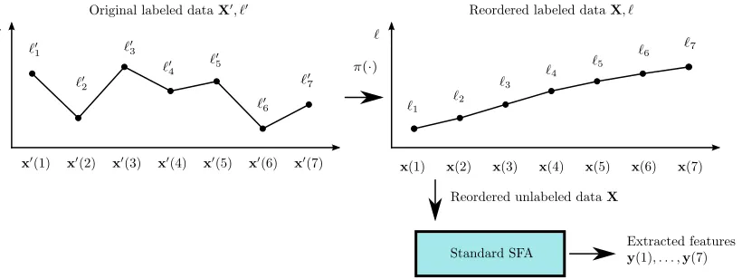
5.1 Sample reordering
LetX0 = (x0(1), . . . ,x0(N)) be a sequence of N data samples with labels`0 = (`01, . . . , `0N). The data is reordered by means of a permutationπ(·) in such a way that the labels become increasing. The reordered samples are X= (x(1), . . . ,x(N)), where x(n) =x0(π(n)), and their labels are`= (`1, . . . , `N) with`l≤`l+1. Afterwards the sequenceX is used to train
standard SFA using the regular single-sequence method (Figure 5).
Figure 5: Sample reordering approach. Standard SFA is trained with a reordered sample sequence, in which the hidden labels are increasing.
Since the ordered label values only increase, they change very slowly and should be found by SFA (or actually some increasing/decreasing function of the labels that also fulfils the normalization conditions). Clearly, SFA could only extract this information if the samples indeed intrinsically contain information about the labels such that it is possible to extract the labels from them. Due to limitations of the feature space considered, insufficient data, noise, etc., one typically obtains noisy and distorted versions of the predicted signals.
In this basic approach, the computation of the covariance matrices takes O(N) oper-ations. Since this method only requires standard SFA and is the most straightforward to implement, we recommend its use for first experiments. If more robust outputs are desired, the methods below based on GSFA are more appropriate.
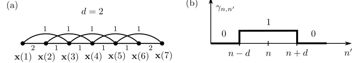
5.2 Sliding window training graph
This is an improvement over the method above in which GSFA facilitates the consider-ation of more connections. Starting from the reordered sequence X as defined above, a training graph is constructed. In this graph, each samplex(n) is connected to its dclosest samples to the left and to the right in the order given by X. Thus, x(n) is connected to the samples x(n−d), . . . ,x(n−1), x(n+ 1), . . . ,x(n+d) (Figure 6.a). In this graph, the vertex weights are constant, i.e., vn = 1, and the edge weights depend on the
dis-tance of the samples involved, that is, ∀n, n0 : γ
n,n0 = f(|n0 −n|), for some function
employ γn,n0 = 2 if (n+n0≤d+ 1 orn+n0 ≥2N−1), γn,n0 = 1 if |n0 −n| ≤ d but not(n+n0 ≤ d+ 1 orn+n0 ≥ 2N −1), and γn,n0 = 0 otherwise. These weights avoid
pathological solutions that sometimes occur if only weights 0 and 1 were used.
Figure 6: (a) A square sliding window training graph with a half-width of d = 2. Each vertex is thus adjacent to at most 4 other vertices. (b) Illustration of the weights of an intermediate nodenfor a square weight window with a half-widthd.
Pathological solutions can occur when a sample is weakly connected to its neighbours. SFA might map such sample to outputs with a large magnitude (to achieve unit variance) and allow for a large difference between its outputs and the outputs of the neighbouring samples (since it is not strongly connected to them). From the normalization constraints of the optimization problem, this results in most samples producing small outputs with almost zero amplitude. Thus, in pathological solutions a large amount of the information about the labels is lost. In practice, these solutions can be prevented, for example, by enforcing the normalization restriction (34) and limiting self-loops on the training graph.
In the sliding window training graph, the computation of CG and C˙G requiresO(dN) operations. If the window is square, the computation can be improved toO(N) operations by using accumulators for sums and products and reusing intermediate results. While larger
d implies more connections, connecting too distant samples is undesired. The selection of
dis non-crucial and done empirically.
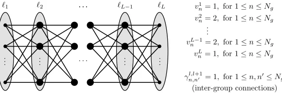
5.3 Serial training graph
Theserial training graph is similar to the clustered training graph used for classification in terms of construction and efficiency. It results from discretizing the original labels` into a relatively small set of discrete labels of sizeL, namely{`1, . . . , `L}, where`1< `2 <· · ·< `L.
As described below, faster training is achieved if Lis small, e.g., 3≤LN.
In this graph, the vertices are grouped according to their discrete labels. Every sample in the group with label `l is connected to every sample in the groups with label `l+1 and `l−1 (except the samples in the first and last groups, which can only be connected to one
neighbouring group). The only existing connections are inter-group connections, no intra-group connections are present.
The samples used for training are denoted by xl(n), where the index l (1 ≤ l ≤ L) denotes the group (discrete label) and n (1 ≤ n ≤ Nl) denotes the sample within such a
group. For simplicity, we assume here that all groups have the same numberNg of samples: ∀l: Nl=Ng. Thus the total number of samples is N =LNg. The vertex weight of xl(n)
of the edge (xl(n),xl+1(n0)) is denoted by γn,nl,l+10 , and we use the same edge weight for all
connections: ∀n, n0, l : γn,nl,l+10 = 1. Thus, all edges have a weight of 1, and all samples are assigned a weight of 2 except for the samples in the first and last groups, which have a weight of 1 (Figure 7). The reason for the different weights on the first and last groups is to avoid pathological solutions and to enforce the normalization restriction (34). Notice that since any two vertices of the same group are adjacent to exactly the same neighbours, they are likely to be mapped to similar outputs by GSFA.
Figure 7: Illustration of a serial training graph with L discrete labels. Even though the original labels of two samples might differ, they will be grouped together if they have the same discrete label. In the figure, a bigger node represents a sample with a larger weight, and the ovals represent the groups.
The sum of vertex weights is Q (13)= Ng + 2Ng(L −2) + Ng = 2Ng(L−1) and the
sum of edge weights is R (12)= (L−1)(Ng)2, which is also the number of connections
con-sidered. Unsurprisingly, the structure of the graph can be exploited to train GSFA effi-ciently. Similarly to the clustered training graph, define the average of the samples from the group l as ˆxl def= P
nxl(n)/Ng, the sum of the products of samples from group l as
Πl=P
nxl(n)(xl(n))T, and the weighted sample average as:
ˆ
x def= 1
Q
X
n
x1(n) +xL(n) + 2
L−1
X
l=2 xl(n)
!
= 1
2(L−1) ˆx
1+ ˆxL+ 2 L−1
X l=2 ˆ xl ! . (60)
From (14), the sample covariance matrix accounting for the weights vnl of the serial training graph is:
Cser (14) = 1 Q X n
x1(n)(x1(n))T + 2
L−1
X
l=2
X
n
xl(n)(xl(n))T +X
n
xL(n)(xL(n))T −Qxˆ(ˆx)T
!
(61)
= 1
Q Π
1+ ΠL+ 2 L−1
X
l=2
Πl−Qxˆ0(ˆx0)T
!
From (16), the matrix C˙G using the edges γn,nl,l+10 defined above is: ˙ Cser (16) = 1 R L−1
X
l=1
X
n,n0
(xl+1(n0)−xl(n))(xl+1(n0)−xl(n))T (63)
= 1
R L−1
X
l=1
X
n,n0
xl+1(n0)(xl+1(n0))T +xl(n)(xl(n))T −xl(n)(xl+1(n0))T −xl+1(n0)(xl(n))T
(64)
= 1
R L−1
X
l=1
X
n0
Πl+1+ Πl− X n
xl(n) X
n0
xl+1(n0)T − X n0
xl+1(n0) X
n
xl(n)T
(65)
= Ng
R L−1
X
l=1
Πl+1+ Πl−Ngxˆl(ˆxl+1)T −Ngxˆl+1(ˆxl)T
. (66)
By using (66) instead of (63), the slowest step in the computation of the covariance matrices, which is the computation of C˙ser, can be reduced in complexity fromO(L(Ng)2)
to only O(N) operations (N = LNg), which is of the same order as the computation of Cser. Thus, for the same number of samplesN, we obtain a larger speed-up for larger group
sizes.
Discretization introduces some type of quantization error. While a large number of discrete labelsLresults in a smaller quantization error, having too many of them is undesired because fewer edges would be considered, which would increase the number of samples needed to reduce the overall error. For example, in the extreme case of Ng = 1 and L = N, this method does not bring any benefit because it is almost equivalent to the sample reordering approach (differing only due to the smaller weights of the first and last samples).
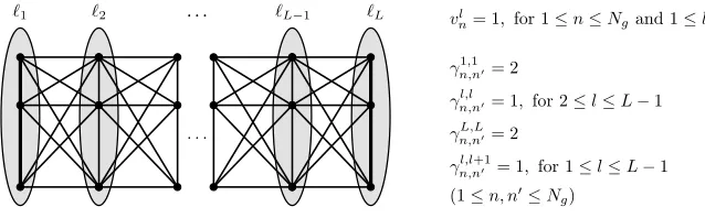
5.4 Mixed training graph
The serial training graph does not have intra-group connections, and therefore the output differences of samples with the same label are not explicitly being minimized. One argument against intra-group connections is that if two vertices are adjacent to the same set of vertices, their corresponding samples are already likely to be mapped to similar outputs. However, in some cases, particularly for small numbers of training samples, additional intra-group connections might indeed improve robustness. We thus conceived themixed training graph (Figure 8), which is a combination of the serial and clustered training graph and fulfils the consistency restriction (34). In the mixed training graph, all nodes and edges have a weight of 1, except for the intra-group edges in the first and last groups, which have a weight of 2. As expected, the computation of the covariance matrices can also be done efficiently for this training graph (details omitted).
5.5 Supervised step for regression problems
Figure 8: Illustration of the mixed training graph. Samples having the same label are fully connected (intra-group connections, represented with vertical edges) and all samples of adjacent groups are connected (inter-group connections). All vertex and edge weights are equal to 1 except for the intra-group edge weights of the first and last groups, which are equal to 2 as represented by wide edges.
as linear or nonlinear regression. The second one is to discretize the original labels to a small discrete set {`˜1, . . . ,`˜L˜} (which might be different from the discrete set used by the
training graphs). The discrete labels are then treated as classes, and a classifier is trained to predict them from the slow features. One can then output the predicted class as the estimated label. Of course, an error due to the discretization of the labels is unavoidable. The third approach improves on the second one by using a classifier that also estimates class membership probabilities. Let P(C˜`
l|y) be the estimated class probability that the input samplexwith slow featuresy=g(x) belongs to the group with (discretized) label ˜`l.
Class probabilities can be used to provide a more robust estimation of a soft (continuous) label `, better suited to the particular loss function. For instance, one can use
` def=
˜ L
X
l=1
˜
`l·P(C˜`l|y) (67)
if the loss function is the RMSE, where the slow featuresymight be extracted using any of the four SFA-based methods for regression above. Other loss functions, such as the Mean Average Error (MAE), can be addressed in a similar way.
We have tested these three approaches in combination with supervised algorithms such as linear regression, and classifiers such as nearest neighbour, nearest centroid, Gaussian classifier, and SVMs. We recommend using the soft labels computed from the class proba-bilities estimated by a Gaussian classifier because in most of our experiments this method has provided best performance and robustness. Of course, other classifiers providing class probabilities could also be used.
6. Experimental Evaluation of the Methods Proposed
6.1 Classification
For classification, we have proposed the clustered training graph. As mentioned in Sec-tion 4.2, when this graph is used, the outputs of GSFA are equivalent to those of FDA. Since FDA has been used and evaluated exhaustively, here we only verify that our imple-mentation of GSFA generates the expected results when trained with such a graph.
The German Traffic Sign Recognition Benchmark (Stallkamp et al., 2011) was chosen for the experimental test. This was a competition with the goal of classifying photographs of 43 different traffic signs taken on German roads under uncontrolled conditions with variations in lighting, sign size, and distance. No detection step was necessary because the true position of the signs was included as annotations, making this a pure classification task and ideal for our test. We participated in the online version of the competition, where 26,640 labeled images were provided for training and 12,569 images without label for evaluation (classification rate was computed by the organisers, who had ground-truth data).
Two-layer nonlinear cascaded (non-hierarchical) SFA was employed. To achieve good performance, the choice of the nonlinear expansion function is crucial. If it is too simple (e.g., low-dimensional), it does not solve the problem; if it is too complex (e.g., high-dimensional), it might overfit to the training data and not generalize well to test data. In all the experiments done here, a compact expansion that only doubles the data dimension was employed, xT 7→ xT,(|x|0.8)T, where the absolute value and exponent 0.8 are
com-puted component-wise. We refer to this expansion as 0.8Exp. Previously, Escalante-B. and Wiskott (2011) have reported that it offers good generalization and competitive performance in SFA networks, presumably due to certain computational properties.
Our method, complemented by a Gaussian classifier on 42 slow features, achieved a recognition rate of 96.4% on test data3 which, as expected, was similar to the reported performance of various methods based on FDA participating in the same competition. For comparison, human performance was 98.81%, and a convolutional neural network gave top performance with a 98.98% recognition rate.
6.2 Regression
The remaining training graphs have all been designed for regression problems and were evaluated with the problem of estimating the horizontal position of a face in frontal face photographs, an important regression problem because it can be used as a component of a face detection system, as we proposed previously (see Mohamed and Mahdi, 2010). In our system, face detection is decomposed into the problems of the estimation of the horizontal position of a face, its vertical position, and its size. Afterwards, face detection is refined by locating each eye more accurately with the same approach applied now to the eyes instead of to the face centers. Below, we explain this regression problem, the algorithms evaluated, and the results in more detail.
6.2.1 Problem and dataset description
To increase image variability and improve generalization, face images from several databases were used, namely 1,521 images from BioID (Jesorsky et al., 2001), 9,030 from CAS-PEAL (Gao et al., 2008), 5,479 from Caltech (Fink et al.), 9,113 from FaceTracer (Ku-mar et al., 2008), and 39,328 from FRGC (Phillips et al., 2005) making a total of 64,471 images, which were automatically pre-processed through a normalization and a reintroduction step. In the first step, each image was converted to greyscale and pose-normalized using annotated facial points so that the face is centered4, has a fixed eye-mouth-triangle area, and the resulting pose-normalized image has a resolution of 256×192 pixels. In the second step, horizontal and vertical displacements were re-introduced, as well as scalings, so that the center of the face deviates horizontally at most ±45 pixels from the center of the image. The vertical position and the size of the face were randomized, so that vertically the face center deviates at most±20 pixels, and the smallest faces are half the size of the largest faces (a ratio of at most 1 to 4 in area). Interpolation (e.g., needed for scaling and sub-pixel displacements) was done using bicubic interpolation. At last, the images were cropped to 128×128 pixels.
Given a pre-processed input image, as described above, with a face at position (x, y) w.r.t. the image center and sizez, the regression problem is then to estimate thex-coordinate of the center of the face. The range of the variables x, yandz is bounded to a box, so that one does not have to consider extremely small faces, for example. To assure a robust estimation for new images, invariance to a large number of factors is needed, including the vertical position of the face, its size, the expression and identity of the subject, his or her accessories, clothing, hair style, the lighting conditions, and the background.
Figure 9: Example of a pose-normalized image (left), and various images after pose was reintroduced illustrating the final range of vertical and horizontal displacements, as well as the face sizes (right).
To increase the usefulness of the images available, each image was pose-normalized once, but pose was reintroduced twice. This results in two post-processed images per original image having different random displacements and scalings. The post-processed images were then randomly split in three datasets (disjoint w.r.t. the original images) to perform particular sub-tasks. The first dataset, containing 30,000×2 images, was used to train the dimensionality reduction method (the factor 2 is due to the double pose-reintroduction
4. The center of a face was defined here as1 4LE+
1 4RE+
1
2M, whereLE,REandMare the coordinates
above). The second one contains 20,000×2 images and was used to train the supervised post-processing step. The third dataset consists of 9,000×2 images and was used for testing.
6.2.2 Dimensionality-reduction methods evaluated
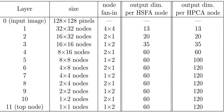
The resolution of the images and their number make it less practical to apply the majority of supervised methods, such as an SVM, and unsupervised methods, such as PCA/ICA/LLE, directly to the images. We circumvent this by using three efficient dimensionality reduc-tion methods, and by applying supervised processing on the lower-dimensional features ex-tracted. The first two methods are efficient hierarchical implementations of SFA and GSFA (referred to as HSFA without distinction). The nodes in the HSFA networks first expand the data using the 0.8Expexpansion function (see Section 6.1) and then apply SFA/GSFA to it, except for the nodes in the first layer in which additionally PCA is applied before the expansion. For comparison, we use a third method, a hierarchical implementation of PCA (HPCA), in which all nodes do pure PCA. The structure of the hierarchies for the HSFA and PCA networks is described in Table 1.
Layer size node output dim. output dim.
fan-in per HSFA node per HPCA node
0 (input image) 128×128 pixels — — —
1 32×32 nodes 4×4 13 13
2 16×32 nodes 2×1 20 20
3 16×16 nodes 1×2 35 35
4 8×16 nodes 2×1 60 60
5 8×8 nodes 1×2 60 100
6 4×8 nodes 2×1 60 120
7 4×4 nodes 1×2 60 120
8 2×4 nodes 2×1 60 120
9 2×2 nodes 1×2 60 120
10 1×2 nodes 2×1 60 120
11 (top node) 1×1 nodes 1×2 60 120
Table 1: Structure of the SFA and PCA deep hierarchical networks. The networks only differ in the type of processing done by each node and in the number of features preserved. For HSFA an upper bound of 60 features was set, whereas for HPCA at most 120 features were preserved.
generic machine learning algorithms for this problem. For the data employed, 120 HPCA features at the top node explain 88% of the data variance, suggesting that HPCA is indeed a good approximation to PCA in this case.
The following dimensionality-reduction methods were evaluated (one based on SFA, four based on GSFA, and one based on PCA).
• SFA using sample reordering (reordering).
• GSFA with a square sliding window graph withd= 16 (SW16).
• GSFA with a square sliding window graph withd= 32 (SW32).
• GSFA with a serial training graph with L= 50 groups of Ng = 600 images (serial).
• GSFA with a mixed graph and the same number of groups and images (mixed).
• A hierarchical implementation of PCA (HPCA).
The evolution across the hierarchical network of the two slowest features extracted by HSFA is illustrated in Figure 10.
6.2.3 Supervised post-processing algorithms considered
On top of the dimensionality reduction methods, we employed the following supervised post-processing algorithms.
• A nearest centroid classifier (NCC).
• Labels estimated using (67) and the class membership probabilities given by a Gaus-sian classifier (Soft GC).
• A multi-class (one-versus-one) SVM (Chang and Lin, 2011) with a Gaussian radial basis kernel, and grid search for model selection.
• Linear regression (LR).
To train the classifiers, the images of the second dataset were grouped in 50 equally large classes according to their horizontal displacement x,−45≤x≤45.
6.2.4 Results
We evaluated all the combinations of a dimensionality reduction method (reordering, SW16, SW32, serial, mixed and HPCA) and a supervised post-processing algorithm (NCC, Soft GC, SVM, LR). Their performance was measured on test data and reported in terms of the RMSE. The labels estimated depend on three parameters: the number of features passed to the supervised post-processing algorithm, and the parametersC andγ in the case of the SVM. These parameters were determined for each combination of algorithms using a single trial, but the RMSEs reported here were averaged over 5 trials.
Figure 10: Evolution of the slow features extracted from test data after layers 1, 4, 7 and 11 of a GSFA network. A central node was selected from each layer, and three plots are provided. i.e.,y2 vsy1,nvsy1, andy2 vs n. This network was trained with
the serial training graph. Notice how slowness improves and structure appears as one moves to higher stages of the network.
graph, GSFA was 4% to 13% more accurate than the basic reordering of samples employing standard SFA. In turn, reordering was at least 10% better than HPCA for this dataset.
Taking a look at the number of features used by each supervised post-processing algo-rithm, one can realize that considerably fewer HSFA-features are used than HPCA-features (e.g., 5 vs. 54 for Soft GC). This can be explained because PCA is sensitive to many factors that are irrelevant to solve the regression problem, such as the vertical position of the face, its scale, the background, lighting, etc. Thus, the information that encodes the horizon-tal position of a face is mixed with other information and distributed over many principal components, whereas it is more concentrated in the slowest components of SFA.
Dim. Reduction NCC # of Soft GC # of SVM # of LR # of
method (RMSE) feat. (RMSE) feat. (RMSE) feat. (RMSE) feat.
Reordering/SFA 6.16 6 5.63 4 6.00 14 10.23 60
SW16 (GSFA) 5.80 5 5.26 5 5.60 17 9.77 60
SW32 (GSFA) 5.75 5 5.25 4 5.51 18 9.73 60
Serial (GSFA) 5.58 4 5.03 5 5.23 15 9.68 60
Mixed (GSFA) 5.63 4 5.12 4 5.40 19 9.54 60
HPCA 29.68 118 6.17 54 8.09 50 19.24 120
Table 2: Performance (RMSE) of the dimensionality reduction algorithms measured in pix-els in combination with various supervised algorithms for the post-processing step. The RMSE at chance level is 25.98 pixels. Each entry reports the best perfor-mance achievable using a different number of features and parameters in the post-processing step. Largest standard deviation of 0.21 pixels. Clearly, linear regression benefitted from all the SFA and PCA features available.
did modestly for HSFA, but even worse than the chance level for HPCA. The SVMs were consistently better, but the error can be further reduced by 4% to 23% by using Soft GC, the soft labels derived from the Gaussian classifier.
Regarding the training graphs, we expected that the sliding window graphs, SW16 and SW32, would be more accurate than the serial and mixed graphs, even when using a square window, because the labels are not discretized. Surprisingly, the mixed and serial graphs were the most accurate ones. This might be explained in part by a larger number of connections in these graphs, or by some type of coupling by the sample groups in them and the classes of the post-processing algorithms. Still, SW16 and SW32 were better than the reordering approach, being the wider window slightly superior. The serial graph was better than the mixed one by less than 2% (for Soft GC), making it uncertain for statistical reasons which one of them is better for this problem. A larger number of trials, or even better, a more detailed mathematical analysis of the graphs might be necessary for this purpose.
7. Discussion
In this paper, we proposed graph-based SFA (GSFA), an implicitly supervised extension of the (unsupervised) SFA algorithm. The main goal of GSFA is to solve supervised learning problems by reducing the dimensionality of the data to a few very label-predictive features. This algorithm is trained with a structure called training graph, in which the vertices are the training samples and the edges represent connections between samples. Edge weights allow the specification of desired output similarities and can be derived from the label or class information.
Therefore, GSFA does not fit to the labels explicitly, but instead fully concentrates on the generation of slow features according to the topology defined by the graph.
We also propose a weighted SFA optimization problem that takes into account the additional edge and weight information contained in a training graph, and generalizes the notion of slowness from a plain sequence of samples to such a graph. Moreover, we prove that GSFA solves the new optimization problem in the function space considered.
The algorithm shares many properties and advantages with its unsupervised coun-terpart, allowing its hierarchical implementation and facilitating the processing of high-dimensional data even when the number of samples is large. Moreover, it can be trained very efficiently in a feed-forward manner layer by layer, and the features at the top node can be complex and highly nonlinear w.r.t. the input. The experimental results demonstrate that the larger number of connections considered by GSFA indeed provides a more robust learning than standard SFA.
Unsupervised dimensionality reduction algorithms extract features that are frequently less useful for the particular supervised problem at hand. For instance, PCA does not yield good features for age estimation from adult face photographs because features revealing age (e.g., skin textures) have higher spatial frequencies and do not belong to the main principal components. Supervised dimensionality reduction algorithms, including GSFA, are more appropriate when one does not know a good set of features for the particular data and problem at hand, and one wants to improve performance by generating features adatpted to the specific data and labels.
Both classification and regression tasks can be solved with GSFA. We showed that a few slow features allow the solution of the supervised learning problem, and require only a small post-processing step that maps the features to labels or classes.
For classification problems, a clustered training graph was proposed, yielding features having the discrimination capability of FDA. The results of the implementation of this graph confirmed the expectations from theory. Training with the clustered graph comes down to considering all transitions between samples of the same identity and no transition between different identities. This is an advantage over Berkes (2005a), where a large number of transitions have to be explicitly considered.
The Markov chain generated through the probabilistic interpretation of this graph is equal to the Markov chain defined by Klampfl and Maass (2010). These Markov chains are parameterized by vanishing parameters and a, respectively. However, the Markov chain and are introduced here for analytical purposes only. In practice, GSFA directly uses the graph structure, which is deterministic and free of . This avoids the inefficient training of SFA with a very long sequence of samples generated with the Markov chain, as done by Klampfl and Maass (2010). (Even though the set of samples if finite, as the parameter a
approaches 0, an infinite sequence is required to properly capture the data statistics of all identities).
future advances in generic methods for SFA, such as hierarchical network architectures or robust nonlinearities, might result in improved classification rates. Of course, it is possible to design other training graphs for classification without this equivalence, e.g., by using non-constant sample weights, or by incorporating input similarity information or other criteria in the edge-weight matrix.
To solve regression problems, we proposed three training graphs for GSFA that resulted in a reduction of the RMSE of up to 11% over the basic reordering approach using standard SFA, an improvement caused by the higher number of similarity relations considered even though the same number of training samples is used.
First extensions of SFA for regression were employed by Escalante-B. and Wiskott (2010) to estimate age and gender from frontal static face images of artificial subjects, created with special software for 3D face modelling and rendering. Gender estimation was treated as a regression problem because the software represents gender as a continuous variable (e.g.,
−1.0=typical masculine face, 0.0=neutral, 1.0=typical feminine face). Early versions of the mixed and serial training graphs were employed. Only three extracted features are passed to an explicit regression step based on a Gaussian classifier (Section 5.5). In both cases, good performance is achieved, with an RMSE of 3.8 years for age and 0.33 units for gender on test data, compared to a chance level of 13.8 years and 1.73 units, respectively.
Using a similar approach, other parameters such as the x-position,y-position, or scale of a face within an image have been estimated (Mohamed and Mahdi, 2010). Using three separate SFA networks, one for each parameter, faces can be pose-normalized. A fourth network can be trained to estimate the quality of the normalization, again as a continuous parameter, and to indicate whether a face is present at all. These four networks together were used to detect faces. Performance of the resulting face detection system on various image databases was competitive and yielded a detection rate on greyscale photographs from 71.5% to 99.5% depending on the difficulty of the test images.
The serial and mixed training graphs provided the best accuracy in this case, with the serial one being slightly more accurate but not to a significant level. These graphs have the advantage over the sliding window graph that they are also suitable for cases in which the labels are discrete from the beginning, which occurs frequently due to the finite resolution in measurements or due to discrete phenomena (e.g., when learning the number of red blood cells in a sample, or a distance in pixels). We are developing a theory on the slowest features that might be extracted by arbitrary graphs. This analysis might solve the question of which one of these two graphs is better or even give rise to a new one.
Although supervised learning is less biologically plausible, GSFA being implicitly su-pervised is still closely connected to feasible unsusu-pervised biological models through the probabilistic interpretation of the graph. If we ensure that the graph fulfils the normaliza-tion restricnormaliza-tions, the Markov chain described in Secnormaliza-tion 3.5 can be constructed, and learning with GSFA and such graph becomes equivalent to learning with standard (unsupervised) SFA as long as the training sequence originates from the Markov chain. From this perspec-tive, GSFA uses the graph information to simplify a learning procedure that could also be done unsupervised.
One limitation of hierarchical processing with GSFA or SFA (i.e., HSFA) is that the features in the data should be spatially localized. For instance, if one randomly shuffles the pixels in the input image performance would decrease considerably. This reduces the applicability of HSFA to scenarios with heterogeneous independent sources of data, but is well suited, for example, for images. Although GSFA makes a more efficient use of the samples available than SFA, it can still overfit in part because these algorithms lack an explicit regularization parameter (although hierarchical processing and certain expansions can be seen as a regularization measures). Hence, for a small number of samples data randomization techniques are useful.
We do not claim that GSFA is better or worse than other supervised learning algorithms. We only show that it is better for supervised learning than SFA, and believe that it is a very interesting and promising algorithm. Of course, specialized algorithms might outperform GSFA for particular tasks. For instance, algorithms for face detection can outperform the system presented here, but a fundamental advantage of GSFA is that it is general purpose. Moreover, various improvements to GSFA (not discussed here) are under development, which will increase its performance and narrow the gap to specialized algorithms.
Most of this work was originally motivated by the need to improve generalization of our learning system. Of course, if the amount of training data and computation time were unrestricted, generalization would be less of an issue, and all SFA training methods would approximately converge to the same features and provide similar performance. Generaliza-tion has different facets, however. For instance, one interpretaGeneraliza-tion is that GSFA provides better performance than SFA (reordering method) using the same amount of training data, as shown in the results. Another interpretation is that GSFA demands less training data to achieve the same performance, thus, indeed contributing to our pursuit of generalization.
References
T. Adali and S. Haykin. Adaptive Signal Processing: Next Generation Solutions. Adaptive and Learning Systems for Signal Processing, Communications and Control Series. John Wiley & Sons, 2010.
P. Berkes. Pattern recognition with slow feature analysis. Cognitive Sciences EPrint Archive (CogPrints), February 2005a. URLhttp://cogprints.org/4104/.
P. Berkes. Handwritten digit recognition with nonlinear fisher discriminant analysis. In
P. Berkes and L. Wiskott. Slow feature analysis yields a rich repertoire of complex cell properties. Journal of Vision, 5(6):579–602, 2005.
A. Bray and D. Martinez. Kernel-based extraction of slow features: Complex cells learn disparity and translation invariance from natural images. In NIPS, volume 15, pages 253–260, Cambridge, MA, 2003. MIT Press.
C.-C. Chang and C.-J. Lin. LIBSVM: A library for support vector machines. ACM Trans-actions on Intelligent Systems and Technology, 2:27:1–27:27, 2011.
A. N. Escalante-B. and L. Wiskott. Gender and age estimation from synthetic face images with hierarchical slow feature analysis. In International Conference on Information Pro-cessing and Management of Uncertainty in Knowledge-Based Systems, pages 240–249, 2010.
A. N. Escalante-B. and L. Wiskott. Heuristic evaluation of expansions for Non-Linear Hier-archical Slow Feature Analysis. In Proc. The 10th International Conference on Machine Learning and Applications, pages 133–138, Los Alamitos, CA, USA, 2011.
A. N. Escalante-B. and L. Wiskott. Slow feature analysis: Perspectives for technical appli-cations of a versatile learning algorithm. K¨unstliche Intelligenz [Artificial Intelligence], 26(4):341–348, 2012.
M. Fink, R. Fergus, and A. Angelova. Caltech 10,000 web faces. URLhttp://www.vision. caltech.edu/Image_Datasets/Caltech_10K_WebFaces/.
R. A. Fisher. The use of multiple measurements in taxonomic problems.Annals of Eugenics, 7:179–188, 1936.
P. F¨oldi´ak. Learning invariance from transformation sequences. Neural Computation, 3(2): 194–200, 1991.
M. Franzius, H. Sprekeler, and L. Wiskott. Slowness and sparseness lead to place, head-direction, and spatial-view cells. PLoS Computational Biology, 3(8):1605–1622, 2007.
M. Franzius, N. Wilbert, and L. Wiskott. Invariant object recognition with slow feature analysis. In Proc. of the 18th ICANN, volume 5163 of LNCS, pages 961–970. Springer, 2008.
M. Franzius, N. Wilbert, and L. Wiskott. Invariant object recognition and pose estimation with slow feature analysis. Neural Computation, 23(9):2289–2323, 2011.
W. Gao, B. Cao, S. Shan, X. Chen, D. Zhou, X. Zhang, and D. Zhao. The CAS-PEAL large-scale chinese face database and baseline evaluations.IEEE Transactions on Systems, Man, and Cybernetics, Part A, 38(1):149–161, 2008.
X. He and P. Niyogi. Locality Preserving Projections. In Neural Information Processing Systems, volume 16, pages 153–160, 2003.
O. Jesorsky, K. J. Kirchberg, and R. Frischholz. Robust face detection using the haus-dorff distance. In Proc. of Third International Conference on Audio- and Video-Based Biometric Person Authentication, pages 90–95. Springer-Verlag, 2001.
S. Klampfl and W. Maass. Replacing supervised classification learning by Slow Feature Analysis in spiking neural networks. In Proc. of NIPS 2009: Advances in Neural Infor-mation Processing Systems, volume 22, pages 988–996. MIT Press, 2010.
P. Koch, W. Konen, and K. Hein. Gesture recognition on few training data using slow feature analysis and parametric bootstrap. In International Joint Conference on Neural Networks, pages 1 –8, 2010.
T. Kuhnl, F. Kummert, and J. Fritsch. Monocular road segmentation using slow feature analysis. In Intelligent Vehicles Symposium, IEEE, pages 800–806, june 2011.
N. Kumar, P. N. Belhumeur, and S. K. Nayar. FaceTracer: A search engine for large collections of images with faces. In European Conference on Computer Vision (ECCV), pages 340–353, 2008.
G. Mitchison. Removing time variation with the anti-hebbian differential synapse. Neural Computation, 3(3):312–320, 1991.
N. M. Mohamed and H. Mahdi. A simple evaluation of face detection algorithms using un-published static images. In 10th International Conference on Intelligent Systems Design and Applications, pages 1–5, 2010.
P. J. Phillips, P. J. Flynn, T. Scruggs, K. W. Bowyer, J. Chang, K. Hoffman, J. Marques, J. Min, and W. Worek. Overview of the face recognition grand challenge. In Proc. of IEEE Conference on Computer Vision and Pattern Recognition, volume 1, 2005.
I. Rish, G. Grabarnik, G. Cecchi, F. Pereira, and G. J. Gordon. Closed-form supervised dimensionality reduction with generalized linear models. InProc. of the 25th ICML, pages 832–839, 2008.
H. Sprekeler. On the relation of slow feature analysis and laplacian eigenmaps. Neural Computation, 23(12):3287–3302, 2011.
H. Sprekeler and L. Wiskott. A theory of slow feature analysis for transformation-based input signals with an application to complex cells. Neural Computation, 23(2):303–335, 2011.
J. Stallkamp, M. Schlipsing, J. Salmen, and C. Igel. The German Traffic Sign Recognition Benchmark: A multi-class classification competition. In International Joint Conference on Neural Networks, pages 1453–1460, 2011.
M. Sugiyama. Local fisher discriminant analysis for supervised dimensionality reduction. In Proc. of the 23rd ICML, pages 905–912, 2006.