R E S E A R C H
Open Access
A general quantum difference calculus
Alaa E Hamza
1*, Abdel-Shakoor M Sarhan
2, Enas M Shehata
2and Khaled A Aldwoah
3*Correspondence:
1Department of Mathematics,
Faculty of Science, Cairo University, Giza, Egypt
Full list of author information is available at the end of the article
Abstract
In this paper, we consider a strictly increasing continuous function
β
, and we present a general quantum difference operatorDβwhich is defined to beDβf(t) = (f(
β
(t)) –f(t))/(β
(t) –t). This operator yields the Hahn difference operator whenβ
(t) =qt+ω
, the Jacksonq-difference operator whenβ
(t) =qt,q∈(0, 1),ω
> 0 are fixed real numbers and the forward difference operator whenβ
(t) =t+ω
,ω
> 0. A calculus based on the operatorDβand its inverse is established.MSC: 39A10; 39A13; 39A70; 47B39
Keywords: quantum difference operator; quantum calculus; Hahn difference operator; Jacksonq-difference operator
1 Introduction
The quantum calculus is known as the calculus without limits. It substitutes the classical derivative by a quantum difference operator which allows to deal with sets of nondiffer-entiable functions. Quantum difference operators have an interesting role due to their applications in several mathematical areas such as orthogonal polynomials, basic hyper-geometric functions, combinatorics, the calculus of variations and the theory of relativity. New results in quantum calculus can be found in [–] and the references cited therein. One type of quantum calculus is the Hahn quantum calculus. In [], Hahn introduced his difference operator, as a tool for constructing families of orthogonal polynomials, which is defined by
Dq,ωf(t) =
f(qt+ω) –f(t)
t(q– ) +ω , t=ω, (.)
whereq∈(, ),ω> are fixed andω=–ωq. The derivative att=ωis defined to be the
usual derivativef(ω) whenever it exists. In [, ], the inverse operator was constructed
and a rigorous analysis of the calculus associated withDq,ωwas given. Hamza and Ahmed, in [], studied the existence and uniqueness of solutions of the Hahn difference equations. Also, in [], they established the theory of linear Hahn difference equations. Hahn quan-tum difference operator unifies two important difference operators. The first is the Jackson
q-difference operator which is defined by
Dqf(t) =
f(qt) –f(t)
t(q– ) , t= , (.)
andDqf() =f(), whereqis a fixed number,q∈(, ). The functionf is defined on a
q-geometric setA⊆R(orC) such that whenevert∈A,qt∈A. See [, ]. The second is
the forward difference operatorDωwhich is defined by
Dωf(t) =
f(t+ω) –f(t)
ω , t∈R, (.)
whereωis a fixed number andω> . We refer the reader also to the interesting book [] by Kac and Cheung who presented theq-calculus and theω-calculus in details, associated with the difference operatorsDqandDω, respectively.
Auch in his PhD thesis [] in (supervised by Lynn Erbe and Allan Peterson) intro-duced the forward difference operator
a,bf(t) =
f(σ(t)) –f(t)
σ(t) –t , (.)
whereσ(t) =at+bwitha≥,b≥ anda+b> , and its inverseρ(t) =t–ab. He definedf
on a mixed time scaleTα:={. . . ,ρ(α),ρ(α),α,σ(α),σ(α), . . .},α>–ba, which is a discrete subset ofR.
In this paper, we introduce a general quantum difference operator defined by
Dβf(t) =
f(β(t)) –f(t)
β(t) –t (.)
for everytwithβ(t)=tandDβf(t) =f(t) whenβ(t) =tprovided thatf(t) exists in the usual sense. Here,β:I−→Iis a strictly increasing continuous function, andf is an arbi-trary function defined, in general, on a subsetI⊆Rwithβ(t)∈Ifor anyt∈I.
Throughout this paperXis a Banach space with norm · , and we denote by
βk(t) :=β◦β◦ · · · ◦β
ktimes
(t) and β–k(t) :=β–◦β–◦ · · · ◦β–
ktimes
(t),
k∈N=N∪ {}, whereNis the set of natural numbers. For convenienceβ(t) =tfor all t∈I.
The general functionβmay be linear or nonlinear. Thenβhas many types according to the number of its fixed points inI. Two classes ofβ can be considered. The first class is the family of allβthat has a unique fixed points∈Iand satisfies the following inequality:
(t–s)
β(t) –t≤ for allt∈I.
The second class is the family of allβthat has a unique fixed points∈Iand satisfies the
following inequality:
(t–s)
β(t) –t≥ for allt∈I.
In the whole paper, we consider all functionsβ that belong to the first class, and give a rigorous analysis of the calculus based onDβ. In this class, the movement of the sequence {βk(t)}
k∈N is towardss. Every choice of the functionβgives a new difference operator. Thus, we can obtain a wide class of quantum difference operators with the corresponding quantum calculi.
The advantage of this study is that it helps and allows us to avoid repetition in proving results once for the Jacksonq-difference operator, once for the Hahn difference operator and once for any difference operator on the formDβwithβin that class.
We organize this paper as follows. In Section , we introduce the definition ofβ -deriv-ative and prove its main properties. For instance, we deduce the chain rule, Leibniz’ for-mula and the mean value theorem. In Section , we introduce theβ-integral and we es-tablish the fundamental theorem ofβ-calculus.
2
β
-differentiationAssume that the function β has only one fixed point s∈I and satisfies the following
condition:
(t–s)
β(t) –t≤ for allt∈I, (.) where the equality holds only ift=s. Here,Iis supposed to be an interval of the real line.
In the following, we introduce two important lemmas in proving our main results.
Lemma . The following statements are true.
(i) The sequence of functions{βk(t)}k∈Nconverges uniformly to the constant function ˆ
β(t) :=son every compact intervalJ⊆Icontainings.
(ii) The series∞k=|βk(t) –βk+(t)|is uniformly convergent to|t–s|on every compact
intervalJ⊆Icontainings.
Proof (i) LetJ= [a,b],s∈J. Ift∈[s,b], then condition (.) impliesβk+(t)≤βk(t) for
allk∈N. So, the sequence{βk(t)}k∈Nis decreasing to the constant functionβˆ(t) =s. By Dini’s theorem{βk(t)}k∈Nis uniformly convergent to the constant functionβˆ(t) on the interval [s,b]. Similarly, we can prove its uniform convergence on [a,s]. Consequently,
the sequence{βk(t)}k∈Nis uniformly convergent on the intervalJ= [a,b]. (ii) We apply Dini’s theorem toSn(t) =
n
k=(βk(t) –βk+(t)),n= , , . . . on both [s,b]
and [a,s] to get the desired result.
The proof of the following lemma is straightforward and will be omitted.
Lemma . If f :I−→Xis continuous at s,then the sequence{f(βk(t))}k∈N converges
uniformly to f(s)on every compact interval J⊆I containing s.
Theorem . If f : I −→ X is continuous at s, then the series
∞
k=(βk(t) –
βk+(t))f(βk(t))is uniformly convergent on every compact interval J⊆I containing s.
Proof LetJ⊆I be a compact interval containings. By Lemma ., there existsk∈N
such that
Thenf(βk(t))< +f(s
)fork≥kandt∈J, which in turn implies that
βk(t) –βk+(t) fβk(t) <βk(t) –βk+(t) + f(s) ∀t∈J,k≥k. (.)
Consider the two sequences
Dn(t) = n
k=
βk(t) –βk+(t)fβk(t) (.)
and
Cn(t) = n
k=
βk(t) –βk+(t) + f(s) . (.)
By Lemma .(ii),Cn(t) is uniformly convergent to|t–s|( +f(s)) onJ.
By the Cauchy criterion, given> , there existsn∈Nsuch that
Cn(t) –Cm(t) < ∀t∈J,n≥m≥n. (.)
By using (.) and (.), we have
Dn(t) –Dm(t) ≤ Cn(t) –Cm(t) < ∀n≥m≥max{n,k}.
Therefore,∞k=(βk(t) –βk+(t))f(βk(t))is uniformly convergent onJ. In the following, we present some examples of special forms ofβ which has one fixed points∈Iand satisfies condition (.).
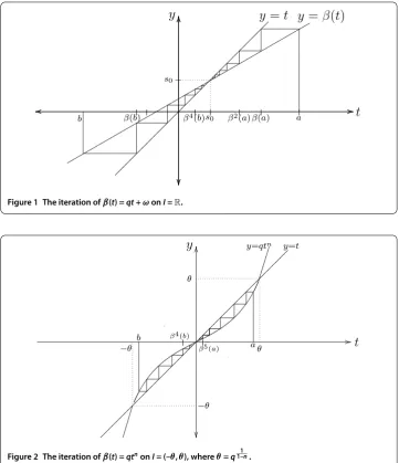
Examples . .β(t) :=qt∓ωfor fixedω≥ andq∈(, ) is defined onI=R. In this case,s=–∓ωq,
βk(t) =qkt∓ω[k]q and β–k(t) =
t±ω[k]q
qk ,
where [k]q=–q k
–q. We have
lim k→∞β
k(t) =s
and lim k→∞β
–k(t) =
∞, t>s,
–∞, t<s
for the iteration ofβ(t) =qt+ωsee Figure .
This case represents both of the forward and backward Hahn difference operators, re-spectively. Also, the Jacksonq-difference operator whenω= , see [–, , ].
.β(t) :=qtnfor fixedq∈(, ) and fixedn∈N+ , andβis defined onI= (–q–n,q–n).
Thenβis a strictly increasing function fromIontoIand has a unique fixed points= ,
andβ–(t) =n t
q. Moreover,
βk(t) =q[k]ntnk, β–k(t) =q–n–k[k]n
Figure 1 The iteration ofβ(t) =qt+ωonI=R.
Figure 2 The iteration ofβ(t) =qtnonI= (–θ,θ), whereθ=q1–1n.
and fort∈I,
lim k→∞β
k(t) = ,
lim k→∞β
–k(t) =
⎧ ⎪ ⎨ ⎪ ⎩
q–n, <t,
, t= , –q–n, t< .
In Figure , we illustrate the behavior ofβk(t) fort∈I. This case yields the power quantum
difference operator
Dn,qf(t) :=
f(qtn)–f(t)
qtn–t , t= ,
f(), t= ,
. Fixn∈N+ ,β(t) :=tnfort∈I= (–, ).β:I−→Iis strictly increasing,β–(t) =√n
t, the unique fixed point iss= ,βk(t) =tn
k
,β–k(t) =t–nk,lim
k→∞βk(t) = fort∈I, and
lim k→∞β
–k(t) =
⎧ ⎪ ⎨ ⎪ ⎩
, t∈(, ), , t= , –, t∈(–, ).
This case represents then-power difference operator []
Dnf(t) :=
f(tn)–f(t)
tn–t , t= ,
f(), t= . (.)
.β(t) :=lnt+ which is a strictly increasing and continuous nonlinear function defined onI= [,∞). The only fixed point iss= . We can see that
βk(t) =lnβk–(t) + , β–(t) =et–,
and fort∈I,
lim k→∞β
k(t) = , lim k→∞β
–k(t) =∞.
Now, we introduce theβ-difference operator as follows.
Definition . For a functionf :I−→X, we define theβ-difference operator off as
Dβf(t) =
f(β(t))–f(t)
β(t)–t , t=s,
f(s), t=s,
provided that the ordinary derivativefexists att=s. In this case, we say thatDβf(t) is theβ-derivative off att. We say thatf isβ-differentiable onIiff(s) exists.
In the following, we state some clear properties of theβ-difference operator.
(i) Dβis a linear operator.
(ii) Iff isβ-differentiable att, thenf(β(t)) =f(t) + (β(t) –t)Dβf(t).
(iii) Iff isβ-differentiable, thenf is continuous ats.
Simple calculations show that the following theorem is true. So, its proof will be omitted.
Theorem . Assume that f :I−→Xand g:I−→Rareβ-differentiable functions at t∈I.Then:
(i) The productfg:I−→Xisβ-differentiable attand
Dβ(fg)(t) =
Dβf(t)
g(t) +fβ(t)Dβg(t) =Dβf(t)
gβ(t)+f(t)Dβg(t).
(ii) f/gisβ-differentiable attand
Dβ(f/g)(t) =
(Dβf(t))g(t) –f(t)Dβg(t)
g(t)g(β(t)) , g(t)g
Examples .
. Dβtn=
n–
k=(β(t))n–k–tk,t∈I,n≥. . Fort= ,Dβt = –tβ(t),t∈I,β(t)= .
. Iff:I−→Rdefined byf(t) = (t, t)andβ(t) =
t+ , then
Dβf(t) =
(–t+t+ , –t)
–t .
. Ifβ(t) =tandf:I−→M×defined byf(t) =
t
t t
, then one can see that
Dβf(t) =
t
t
, whereM×is the space of all×matrices.
Lemma . Let f:I−→Xbeβ-differentiable and Dβf(t) = for all t∈I,then f(t) =f(s), t∈I.
Proof SinceDβf(t) = ,t∈I, thenf(t) =f(β(t)),t∈I. Consequently,f(t) =f(βk(t)),t∈I andk∈N. Takingk→ ∞and using the continuity off ats, we obtainf(t) =f(s) for
t∈I.
As a direct consequence we obtain the following corollary.
Corollary . Suppose that f,g:I−→Xareβ-differentiable on I.If Dβf(t) =Dβg(t)for
all t∈I,then f(t) –g(t) =f(s) –g(s)for all t∈I.
Definition . Lets∈[a,b]⊆I. We define theβ-interval by
[a,b]β=
βk(a);k∈N
∪βk(b);k∈N
∪ {s},
and the class [c]βfor any pointc∈Iby
[c]β=
βk(c);k∈N
∪ {s}.
Finally, for any setA⊂R, we define
A∗=A\ {s}.
In the following lemma, [a,b] is a compact subinterval ofIands∈[a,b].
Lemma . Let f : [a,b]−→Rbe continuous at s.The following statements are true: (i) Dβf(t) > for allt∈[a,b]∗βif and only iff is strictly increasing on[a,b]β.
(ii) Dβf(t) < for allt∈[a,b]∗βif and only iff is strictly decreasing on[a,b]β.
Proof We prove only the first part and the second one can be shown similarly. For the proof of (i), supposeDβf(t) > for allt∈[a,b]∗β. We may assume thats∈ {/ a,b}. We have
a<β(a) <β(a) <· · ·<βk(a) <· · ·<s<· · ·<βm(b) <· · ·<β(b) <b. Then, using the
con-tinuity off ats, we conclude thatf(a) <f(β(a)) <f(β(a)) <· · ·<f(βk(a)) <· · ·<f(s) <
f(βk+(t)) >f(βk(t)), and ifβk+(t) <βk(t), thenf(βk+(t)) <f(βk(t)). Therefore,D
βf(t) > for allt∈[a,b]∗β.
The following example shows that the previous lemma may not hold on [a,b]\[a,b]β.
Example . Letf : [,]−→Rdefined byf(t) = t– t and letβ(t) = t+. One can see thatDβf(t) < ,t∈[,) ands= . Lett= . <t= ., thenf(t) = –. < f(t) = –., which means thatfis not strictly decreasing on the interval [,]. Note that t,t∈/[,]β.
Simple calculations, using induction onm, show that the following theorem is true. So its proof will be omitted.
Theorem . Letαbe a constant and m∈N.
(i) Iff(t) = (t–α)m,then
Dβf(t) =
m–
r=
β(t) –αr(t–α)m––r. (.)
(ii) Ifg(t) = /(t–α)m,then
Dβg(t) = –
m– r=
(β(t) –α)m–r(t–α)r+, (.)
provided that(β(t) –α)m–r(t–α)r+= ,r= , , . . . ,m– .
The following example shows that the ordinary chain rule does not hold in theβ -cal-culus.
Example . Consider the functionsf(t) =tandg(t) = t. Then
Dβ(f◦g)(t) =
β(t) +t,
while
Dβf
g(t)Dβg(t) =
β(t) + t. (.)
That is,
Dβ(f◦g)(t)=Dβf
g(t)Dβg(t). (.)
The next theorem gives us an analogous formula of the chain rule forβ-calculus.
Theorem . Let g:I−→Rbe a continuous andβ-differentiable function and f :R−→
Xbe continuously differentiable.Then there exists a point c betweenβ(t)and t such that
Dβ(f◦g)(t) =f
Proof The caset=sis the usual chain rule. The caset=swithg(β(t)) =g(t) is evident
In the following theorem, we derive the formula for thenthβ-derivative of the product
fg, where one of them is a real-valued function and the other is a vector-valued function. Forn∈N, letSk(n)be the set of all possible strings of lengthncontainingktimesβand
n–ktimesDβ. We denotefDββ(t) = (Dβf)(β(t)) andfβDβ(t) =Dβ(f(β(t))), andfis defined accordingly for∈S(kn).
Iff isβ-differentiablentimes overI, then the higher order derivatives off are defined by
Finally, one can see that
∈S(kn)
Theorem .(Leibniz’ formula) If f and g are n timesβ-differentiable functions,then we have
=
The following example shows that the functionf may be discontinuous but it isβ -differ-entiable.
We see that the functionf is discontinuous but it isβ-differentiable, where
Rolle’s theorem, in general, is not true with respect to the β-derivative. This can be shown by the following example.
Example . The functionf(t) = t– t, defined in Example ., is ordinary
differ-entiable and henceβ-differentiable overRwith respect toβ(t) = t+. Clearly,f() =
f(β()), butf(t)=f(β(t)) inside the interval [,β()],i.e., there are no points between andβ() such thatDβf(t) = . In fact,f(t) =f(β(t)) only at and. This implies the failure of Rolle’s theorem with respect to theβ-derivative.
In the following theorem, we obtain analogues for the classical mean value theorem. We postpone the proof of this theorem to Section .
Theorem .(Mean value theorem) Suppose f,g:I−→Xareβ-differentiable functions on I.Then
f(y) –f(x) ≤sup t∈I
Dβf(t) (y–x) (.)
for every x,y∈[a,b]β,x<s<y,where a,b∈I,a≤b.
The following example shows that inequality (.) does not hold withx,y∈/[a,b]β,x<
s<yanda,b∈I,a≤b.
Example . Letf,g:I= [–, ]−→Rdefined byf(t) =t andg(t) = t andβ(t) =
t+
. Thens= and one can see that|Dβf(t)|<Dβg(t) for allt∈I. If we takea=b= –,
then
[–]β=
,
n–
n :n= –, , , . . .
.
Letx,y∈[–]β,x<y. By Theorem .,|y–x| ≤(y–x) for everyx,y∈[–]β,x<y, wheresupt∈I|Dβf(t)|=. Now, if we takex,y∈/[–]β, wherex= andy=. One can see that|y–x|>
(y–x).
3
β
-integrationWe say thatFis aβ-antiderivative of the functionf :I−→XifDβF(t) =f(t) fort∈I.
Definition . We denote by the vector space of all functions g:I→Xwhich are continuous atsand vanish ats. Define the operatorTβ:−→by
Tβ(g)(t) =g
β(t), t∈I.
LetY be the range ofI–Tβ, whereI is the identity operator. One can check that for
g∈Y the series∞k=g(βk(t)) is uniformly convergent onI. Clearly, the operatorI–Tβ is one-to-one.
Lemma . The operator A:Y−→defined by
A(g)(t) = ∞
k=
gβk(t) (.)
is the inverse of the operatorI–Tβ.
Theorem . Assume f :I→Xis continuous at s.Then the function F defined by
F(t) = ∞
k=
βk(t) –βk+(t)fβk(t), t∈I (.)
is aβ-antiderivative of f with F(s) = .Conversely,aβ-antiderivative F of f vanishing at sis given by formula(.).
Proof For allt∈Iandt=s, we have
DβF(t) =
F(β(t)) –F(t) β(t) –t
=
∞
k=(βk+(t) –βk+(t))f(βk+(t)) –
∞
k=(βk(t) –βk+(t))f(βk(t))
β(t) –t
=f(t).
To show thatDβF(s) =f(s), let> . By the continuity off(t) att=s, there isδ> such
that
fβk(s+h)
–f(s) <, k≥, <h<δ.
This implies
hF(s+h) –f(s)
≤
∞
k=
h
βk(s+h) –βk+(s+h) f
βk(s+h)
–f(s)
<, <h<δ.
Conversely, assume thatFis aβ-antiderivative off vanishing ats. This implies that
f(t) =DβF(t) =
F(β(t)) –F(t) β(t) –t
=Tβ(F(t)) –F(t) β(t) –t
=(I–Tβ)F(t)
t–β(t) .
have
Proof The proof is straightforward.
By Theorem ., we obtain the first fundamental theorem ofβ-calculus which is stated as follows.
Theorem . Let f :I−→Xbe continuous at s.Define the function
F(x) =
x s
f(t)dβt, x∈I. (.)
Then F is continuous at s,DβF(x)exists for all x∈I and DβF(x) =f(x).
Corollary . If f :I−→Xis continuous at s.Then
β(t) t
f(τ)dβτ=
β(t) –tf(t), t∈I. (.)
Proof LetF(t) =st
f(τ)dβτ,t∈I. By Theorem .,F(t) is continuous atsandDβF(t) =
f(t) for allt∈I. Then
β(t) t
f(τ)dβτ=
β(t) s
f(τ)dβτ–
t s
f(τ)dβτ
=Fβ(t)–F(t).
SinceF(β(t)) =F(t) + (β(t) –t)DβF(t), then
β(t) t
f(τ)dβτ=
β(t) –tf(t), t∈I.
Now, we state and prove the second fundamental theorem ofβ-calculus.
Theorem . If f :I−→Xisβ-differentiable on I,then
b a
Dβf(t)dβt=f(b) –f(a) for all a,b∈I. (.)
Proof We have
b s
Dβf(t)dβt= ∞
k=
βk(b) –βk+(b)(Dβf)
βk(b)
= ∞
k=
fβk(b)–fβk+(b)
= lim n→∞
n
k=
fβk(b)–fβk+(b)
Similarly,
a s
Dβf(t)dβt=f(a) –f(s).
Therefore,
b a
Dβf(t)dβt=f(b) –f(a) for alla,b∈I.
As a direct consequence of Theorem ., one can see that the following theorem is true.
Theorem . If f :I−→Xis continuous at sand:I−→Xis aβ-antiderivative of f on I,then for a,b∈I,we have
b a
f(t)dβt=(b) –(a).
The following theorem establishes the formula for theβ-integral by parts. The proof is straightforward, so it will be omitted.
Theorem . Assume f,g areβ-differentiable functions on I and Dβf,Dβg both
contin-uous at s.Then
b a
f(t)Dβg(t)dβt=f(b)g(b) –f(a)g(a) –
b a
Dβf(t)
gβ(t)dβt, a,b∈I.
Here,at least one of the functions f and g is a real-valued function.
The following two lemmas and Definition . are fundamental in the study of the calcu-lus of variations. The first is based originally on [], Lemma . and the second on [], Lemma .. Both are adapted in [] for the case of Hahn’s functionβ(t) =qt+ω,q∈(, ), ω> . Here, following [], we show that both lemmas are valid for the case of our general functionβ(t).
LetDdenote the set of all real-valued functions defined on [c,d]βand continuous ats,
wherec,d∈Iandc<d.
Lemma . Let f ∈D.Then dcf(t)h(β(t))dβt= for all functions h∈D with h(c) =
h(d) = if and only if f(t) = for all t∈[c,d]β.
Proof It is obvious from the definition ofβ-integration that iff(t) = for allt∈[c,d]β, thendcf(t)h(β(t))dβt= . To prove the other implication, assume on the contrary that there is somel∈[c,d]βsuch thatf(l)= . We have the following two cases.
Case I:l=s. Then eitherl=βk(c) orl=βk(d) for somek∈N. First, assume thatl=
βk(c) for somek∈N
. Define
h(t) =
Following [], Lemma ., we show that their results hold for our general functionβ(t).
+ ∞
k=
βk+k+(x) –βk+k(x) fβk+k(x)
≤ ∞
k=
βk+k(y) –βk+k+(y)gβk+k(y)
– ∞
k=
βk+k(x) –βk+k+(x)gβk+k(x)
=
y s
g(t)dβt–
x s
g(t)dβt=
y x
g(t)dβt.
Puttingf(t) = in (.) and (.) we getsy
g(t)dβt≥ and
y
xg(t)dβt≥.
Lemma . Let f :I−→Xand g:I−→Rbeβ-differentiable on I.If
Dβf(t) ≤Dβg(t), t∈[a,b]β,a,b∈I and a≤b,
then
f(y) –f(x) ≤g(y) –g(x) (.)
for every x,y∈[a,b]β,x<s<y.
Proof AssumeDβf(t) ≤Dβg(t),t∈[a,b]β,a,b∈I, a≤b. By Theorem . and Lem-ma . we obtain
xyDβf(t)dβt
≤
y x
Dβg(t)dβt,
which leads to
f(y) –f(x) ≤g(y) –g(x).
We are now in a position to prove Theorem ..
Proof of Theorem . Define the functiong by g(t) =supτ∈IDβf(τ)(t–x). We have
Dβg(t) =supτ∈IDβf(τ) ≥supτ∈[a,b]βDβf(τ) ≥ Dβf(t), t∈[a,b]β. Then, by
Lem-ma .,
f(y) –f(x) ≤g(y) –g(x) =sup t∈I
Dβf(t) (y–x).
4 Conclusion and perspectives
In this paper, we presented a general quantum difference operator Dβf(t) = f(ββ((tt))–)–ft(t), whereβis a strictly increasing continuous function defined onI⊆Rwhich has only one fixed points∈I. This operator yields the Hahn difference operator whenβ(t) =qt+ω,
There is still a lot of work ahead of us. In one direction, we should establish existence and uniqueness results of solutions of difference equations based onDβ (β-difference equa-tions). Another direction is to establish the theory of linear quantum difference equations associated withDβ. Finally, we should ask about the stability of such equations. The the-ory ofβ-difference equations helps and allows us to avoid proving results more than one time, once forq-difference equations, once for Hahn difference equations and once for any choice ofβ.
Competing interests
The authors declare that they have no competing interests.
Authors’ contributions
All authors contributed equally and significantly in writing this paper. All authors read and approved the final manuscript.
Author details
1Department of Mathematics, Faculty of Science, Cairo University, Giza, Egypt.2Department of Mathematics, Faculty of
Science, Menoufia University, Shibin El-kom, Egypt.3Department of Mathematics, Faculty of Science, Islamic University of
Madinah, Al Madinah Al Munawarah, Saudi Arabia.
Acknowledgements
The authors sincerely thank the referees for their valuable suggestions and comments.
Received: 10 November 2014 Accepted: 26 May 2015
References
1. Aldwoah, KA, Malinowska, AB, Torres, DFM: The power quantum calculus and variational problems. Dyn. Contin. Discrete Impuls. Syst., Ser. B, Appl. Algorithms19, 93-116 (2012)
2. Annaby, MH, Hamza, AE, Aldwoah, KA: Hahn difference operator and associated Jackson-Nörlund integrals. J. Optim. Theory Appl.154, 133-153 (2012)
3. Annaby, MH, Mansour, ZS:q-Fractional Calculus and Equations. Springer, Berlin (2012)
4. Hamza, AE, Ahmed, SM: Existence and uniqueness of solutions of Hahn difference equations. Adv. Differ. Equ.2013, 316 (2013)
5. Hamza, AE, Ahmed, SM: Theory of linear Hahn difference equations. J. Adv. Math.4(2), 441-461 (2013) 6. Malinowska, AB, Torres, DFM: The Hahn quantum variational calculus. J. Optim. Theory Appl.147, 419-442 (2010) 7. da Cruz, B, Artur, MC: Symmetric Quantum Calculus. PhD thesis, Aveiro University (2012)
8. Tariboon, J, Ntouyas, SK: Quantum calculus on finite intervals and applications to impulsive difference equations. Adv. Differ. Equ.2013, 282 (2013)
9. Hahn, W: Über orthogonalpolynome, dieq-differenzengleichungen genügen. Math. Nachr.2, 4-34 (1949) 10. Aldwoah, KA: Generalized Time Scales and the Associated Difference Equations. PhD thesis, Cairo University (2009) 11. Bangerezako, G: An Introduction toq-Difference Equations, Bujumbura (2008)
12. Kac, V, Cheung, P: Quantum Calculus. Springer, New York (2002)
13. Auch, TJ: Development and Application of Difference and Fractional Calculus on Discrete Time Scales. PhD thesis, University of Nebraska-Lincoln (2013)