Numerical modeling of the global ionospheric effects of storm sequence on
September 9–14, 2005—comparison with IRI model
M. V. Klimenko1,2, V. V. Klimenko1, K. G. Ratovsky3, and L. P. Goncharenko4
1N.V. Pushkov IZMIRAN RAS, West Department, Kaliningrad, 236010, Russia 2Kaliningrad State Technical University, Kaliningrad, Russia 3Institute of Solar-Terrestrial Physics SB RAS, Irkutsk, Russia
4Haystack Observatory, Massachusetts Institute of Technology, Westford, Mass., U.S.A.
(Received May 31, 2010; Revised April 14, 2011; Accepted June 27, 2011; Online published July 27, 2012)
This study presents the modeling of ionospheric response to geomagnetic storms of September 9–14, 2005. We examine the performance of the Global Self-Consistent Model of Thermosphere, Ionosphere and Protonosphere (GSM TIP) and International Reference Ionosphere-2000 (IRI-2000), and compare the modeling predictions with the ionosonde and incoherent scatter radar observations over Yakutsk, Irkutsk, Millstone Hill and Arecibo stations. IRI-2000 predicted well all negative foF2 disturbances. In comparison with IRI-2000, the GSM TIP
better reproduced the positive phase observed during the disturbed times. We discuss the possible reasons of the differences between the GSM TIP model calculations, IRI predictions, and the observations.
Key words:Ionospheric storm, foF2disturbances, thermospheric wind, neutral atmosphere composition, electric
field, numerical modeling, IRI model.
1.
Introduction
A large number of studies were devoted to modeling of the ionospheric effects of geomagnetic storms (see, e.g., a review by Buonsanto (1999) and references in Klimenkoet al.(2011)). The use of numerical modeling for the descrip-tion of the ionospheric behavior during geomagnetic distur-bances allows investigation of the physical mechanisms re-sponsible for the ionospheric disturbances. In this paper, we discuss the role of each possible mechanism of ionospheric disturbance during geomagnetic storms. A physical mecha-nism for positive ionospheric storms has recently been sug-gested by Balanet al.(2009, 2010). Note that Balanet al.
(2009, 2010) used empirical models of the thermospheric parameters and the measured electric fields as input param-eters for their ionospheric model. Such an approach takes into account the influence of the thermospheric parameters and electric field on the behavior of ionospheric parameters. However, such study does not consider the inverse effect (i.e., the ionospheric influence on the thermospheric param-eters and on the electric field), which in some cases may be very important. The magnetospheric processes act to produce a number of interesting ionospheric features, in-cluding electron and ion temperature hot spots, large-scale plasma blobs, extended tongues of ionization, ionization troughs and peaks, and super plasma fountain. These iono-spheric features then affect the thermoiono-spheric structure, cir-culation, and composition owing to ion-neutral momentum and energy coupling, and these changes, in turn, affect the
Copyright cThe Society of Geomagnetism and Earth, Planetary and Space Sci-ences (SGEPSS); The Seismological Society of Japan; The Volcanological Society of Japan; The Geodetic Society of Japan; The Japanese Society for Planetary Sci-ences; TERRAPUB.
doi:10.5047/eps.2011.06.048
ionosphere (Schunk, 1990). However, the impact of the ionosphere on the neutral density and wind structures is not well understood. A fully self-consistent thermosphere-ionosphere-electrodynamics model is required for a com-prehensive understanding and modeling capability of the impact of the ionosphere on neutral density and wind struc-tures (Forbes, 2007). The simulation results (Maruyama
et al., 2003) suggested that ion drag parallel to the field lines, in the vicinity of a pronounced equatorial ionization anomaly, has a significant impact on the latitudinal struc-ture of the equatorial neutral wind and on the temperastruc-ture structure. Fully self-consistent thermosphere-ionosphere-electrodynamics models were used recently (e.g., Luet al., 2008; Klimenkoet al., 2011) for understanding of forma-tion mechanisms of ionospheric disturbances during geo-magnetic storms.
In parallel to physics-based models investigating the ionospheric effects of geomagnetic storms, empirical mod-els have been developed. The well-known Interna-tional Reference Ionosphere model (IRI-2000) (Bilitza, 2001, 2003) contains a geomagnetic activity dependence based on an empirical storm-time ionospheric correction model. In the present paper we examine both the Global Self-Consistent Model of the Thermosphere, Ionosphere, Protonosphere (GSM TIP) (Namgaladzeet al., 1988, 1991) calculations and the IRI-2000 predictions of the ionospheric effects of the September 9–14, 2005 geomagnetic storm sequence by comparison with experimental data at differ-ent latitudes and longitudes. For this purpose we have se-lected the ionosonde and Incoherent Scatter Radar (ISR) (where available) observations at Yakutsk, Russia (62.0◦N, 129.4◦E; geomagnetic coordinates 51.1◦, 194.2◦), Irkutsk, Russia (52.2◦N, 104.2◦E; geomagnetic coordinates 40.9◦,
175.1◦), Millstone Hill, U.S.A. (42.6◦N, 71.5◦W; geomag-netic coordinates 54.0◦, 357.9◦), and Arecibo, Puerto Rico (18.3◦N, 66.8◦W; geomagnetic coordinates 29.7◦, 3.3◦).
2.
Basic Physical Mechanisms of Ionospheric
Dis-turbances
It is well known that the primary formation mechanisms of ionospheric disturbances are due to the variations in the electric fields and in the thermospheric parameters. Accord-ing to the pioneerAccord-ing work by Mayr and Volland (1973), the middle latitude positive ionospheric disturbances are formed by the meridional component of the thermospheric wind, and the negative disturbances are due to the thermo-sphere composition variations.
It is also known (Rishbeth and Garriott, 1969) that the occurrence of the additional eastward (westward) electric field leads to the additional electromagnetic drift directed to pole and upward (to equator and downward) in the plane of the geomagnetic meridian, and to the plasma transport upward (downward) to the larger (lower) heights into the region of smaller (larger) rates of chemical losses that lead to the positive (negative) effects in the ionosphericF-region electron density.
The appearance of the additional meridional electric field leads to the zonal electromagnetic plasma drift. A poleward electric field leads to a westward plasma drift, and an equa-torward electric field causes a eastward plasma drift. The zonalE×Bdrift leads to a change in the electron density in theF-region of the ionosphere only in locations with lon-gitudinal gradients in the electron density (Klimenko and Namgaladze, 1980). The magnitude of effects in the elec-tron density will depend on the magnitude of these gradi-ents. The most significant effect of the meridional electric field is expected near the solar terminator.
Since the F-region plasma is magnetized it can move across geomagnetic field lines only under the action of an electric field, the effects of which are considered above. Be-cause of the inclination of geomagnetic field to the Earth’s surface the meridional component of thermospheric wind can move the plasma due to ion-neutral collisions, trans-porting it upwards (downwards) along geomagnetic field lines into the regions of lower (larger) chemical loss rates in ion-molecular reactions and leading to the growth (de-crease) in electron density (Rishbeth and Garriott, 1969).
As the atomic oxygen is the primary source of ioniza-tion at F-region heights, and the molecular nitrogen is the primary source of recombination, the change of the
n(O)/n(N2)ratio controls the electron density. The growth
(reduction) of this ratio leads to the positive (negative) dis-turbances in electron density at heights of the ionospheric
F-region (Rishbeth and Garriott, 1969).
Recent modeling results have shown that the additional eastward electric field such as prompt penetration on its own is unlikely to cause positive ionospheric storms (e.g., Balan
et al., 2009). According to the mechanism suggested by Balanet al.(2010), an equatorward neutral wind is required to produce positive ionospheric storms. The mechanical ef-fects of the wind are: (1) to reduce (or stop) the downward diffusion of plasma along the geomagnetic field lines; (2) to raise the ionosphere to higher altitudes with reduced
chem-ical loss; and hence accumulate the plasma at altitudes near and above the ionospheric peak centered at around±30◦ magnetic latitudes. Daytime eastward prompt penetration electric fields, if they occur, also shift the Equatorial Ion-ization Anomaly (EIA) crests to higher than normal lati-tudes. The difference between the earlier and recent mod-elling is in latitudinal coverage: the earlier modmod-elling (e.g., Buonsanto, 1999) considered the effects at high- and mid-latitudes alone, while Balanet al. (2009) considered low-and mid-latitudes.
3.
Description of the Modeled Event and
State-ment of the Problem
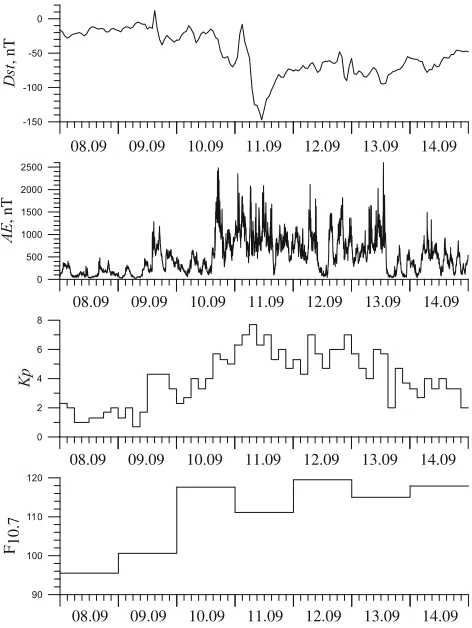
This paper is focused on studies of the ionospheric effects of the September 9–14, 2005 storm sequence. During this period there were several geomagnetic storms following one another: a minor storm on September 9 (Kp = 4+),
a moderate storm on September 10 (Kp=6−), and a major
storm on September 11 (Kp =8−). Figure 1 describes the
behavior of theKp-, AE-, and Dstindices of geomagnetic
activity and the index of the solar activity level, F10.7 for
the period of 8–14 September 2005. It is important to note the high flare activity during the considered period; there were 5 flares on the Sun (on 10 September at 19:10 UT and 21:30 UT, on 11 September at 12:44 UT, on 13 September at 19:19 UT, and on 14 September at 10:05 UT). The considered events occurred at average level of solar activity (F10.7 ∼101–120).
We use the observations from the ionosondes at Irkutsk and Yakutsk and the ISRs at Millstone Hill and Arecibo. All ionosonde ionogram data have been manually scaled us-ing an interactive ionogram scalus-ing software, SAO Explorer (Khmyrovet al., 2008; Reinisch and Galkin, 2011). In ex-perimental data, we use the diurnal variation on 8 Septem-ber 2005 as a quiet-time reference (quiet day) for the ISR observations and the monthly median diurnal variation in the case of the ionosonde data.
dur-Fig. 1. The behavior ofKp-,AE- andDst-index of geomagnetic activity and the index of solar activityF10.7on September, 8–14, 2005.
ing these geomagnetic storms.
The model run presented here is the same as the one de-scribed in detail by Klimenkoet al.(2011). The GSM TIP simulation uses as initial condition the values of ionospheric parameters at 06:00 UT on September 9, 2005, obtained for quiet geomagnetic conditions (Kp =0.7). To calculate the
quiet-time behavior of ionospheric parameters, we varied only the F10.7 index, while the value of the Kp-index
re-mained fixed at the level of 0.7. For quiet conditions, the cross-polar cap potential difference was set equal to 35.7 kV at geomagnetic latitudes±75◦, and R2 FAC, j2,
were set equal to 3×10⁻⁸ A/m2 at geomagnetic latitudes
±70◦. We are setting the maximum and minimum of elec-tric potential rather than potential difference in the latitudi-nal circles of±75◦. The distribution of electric potential is defined in such manner that the electric field in the po-lar cap was directed from dawn to dusk. To be precise, on the dawn side it was set to 17.85 kV, and at the dusk side to−17.85 kV. The electric potential at the latitudinal cir-cle±75◦ varies like a sine function. The zeros of this sine function occur on the day and night sides.
In the GSM TIP storm time calculations, several input parameters such as cross-polar cap potential difference, R2 FAC, and auroral particle precipitations varied as a function of the Kp-index. The cross-polar cap potential difference
was set according to the relation=26.4+13.3×Kp
(kV) (Feshchenko and Maltsev, 2003) at geomagnetic lati-tudes±75◦. Using the morphological results of Iijima and Potemra (1976) and Kikuchi et al. (2008) we have
con-structed the empirical dependences of R2 FAC amplitudes from theKp-index during geomagnetic storms: j2=2.78×
10−8+0.32×10⁻⁸×K
p(A/m2). We also have included the
30 min time delay of R2 FAC variations with respect to the variations of the cross-polar cap potential difference during the storm (Kikuchiet al., 2008). The flux of precipitating auroral electrons is increased and their spectrum becomes harder with growth of geomagnetic activity. The ratio of the precipitating particles fluxes under the storm and quiet time conditions varied as FluxStorm/FluxQuiet=0.55+0.64×Kp.
The GSM TIP model also accounts for the changes in the position of the R2 FAC and high-energy particle precipita-tion during disturbed condiprecipita-tions. We varied the geomag-netic latitudes of the R2 FAC maximum depending on the changes of a cross-polar cap potential difference: 1)±70◦ atKp ≤ 3; 2)±65◦ at 3 < Kp ≤ 6; 3) ±60◦ at 6 < Kp
according to the conclusions of Sojkaet al.(1994). We also introduced the shift of the storm-time precipitation maxi-mum from the local midnight sector into the local morning sector, and the 30 min delay between the particle precipita-tion and the changes of cross-polar cap potential difference. The changes of the polar cap sizes and positions were not taken into account in the GSM TIP model since their in-clusion requires development of an absolutely new model. This is related to the tilted dipole approximation of the Earth’s magnetic field in the GSM TIP model. Geomag-netic field lines in the polar caps are assumed open, while other geomagnetic field lines are closed. The integration of modeling equations for the thermal plasma of theF-region ionosphere and plasmasphere in the GSM TIP model is per-formed along geomagnetic field lines. For the development of the GSM TIP model the grid of the geomagnetic field lines has been kept fixed. Displacement of the equatorial boundary of the polar cap to the equator should automati-cally lead to the expansion of the open geomagnetic field lines. The modeling equations solution on open field lines must be consistent with the boundary conditions, describing the regime of the continual escape of thermal plasma (po-lar wind). The model does not provide the replacement of closed field lines by the open field lines due to the chosen fixed grid. Errors associated with the use of fixed polar cap sizes exist and are not easy to quantify. However, we expect these errors to be not substantial.
4.
Modeled Results and Observations
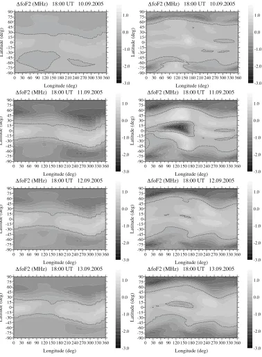
The effects on September 9 and 14 are smaller than in other days, therefore, we restricted data presentation to ionospheric effects during the period from 10 to 14 Septem-ber 2005. Figure 2 shows the global disturbances in the ionospheric F2-layer critical frequency, foF2, obtained by
Fig. 2. The global foF2disturbances obtained in IRI-2000 model (left panel) and in the model GSM TIP (right panel) during the geomagnetic storm sequence on 10, 11, 12 and 13 September, 2005 at 18:00 UT (from top to bottom).
these positive disturbances in both northern and southern hemispheres is∼15–25◦wider in GSM TIP than in the IRI-2000 model. The GSM TIP model also simulates a com-plex longitudinal structure in positive disturbances, while the IRI-2000 predicted response is mostly symmetric with regards to geomagnetic latitude. The GSM TIP simulation results also show a stronger dependence of positive distur-bances on the magnitude of geomagnetic storm, with max-imum positive disturbances in foF2 expected on
Septem-ber 11, 2005. The area of negative disturbances seen in the GSM TIP at equatorial and low latitudes is absent in the IRI-2000 band, but coincides with the area of the reduction of the IRI-2000 predicted positive disturbances at the
geo-magnetic equator.
Figure 3 shows the GSM TIP calculations and IRI-2000 prediction of foF2for quiet and storm conditions over
dif-ferent mid-latitude stations. The three upper rows show the
foF2 variations above the stations of the Eastern-Siberian
longitudinal chain Norilsk (69.4N, 88.1E), Yakutsk (62.0N, 129.4E) and Irkutsk (52.2N, 104.2E). For September 10, the IRI-2000 model predicts negative foF2 disturbances
above Yakutsk and Irkutsk stations, whereas GSM TIP in-dicates the negative foF2disturbances in the afternoon and
the positive disturbances during the night. According to both models, negative foF2disturbances are formed above
Fig. 3. The calculation results of foF2above stations Norilsk, Yakutsk, Irkutsk, Millstone Hill and Arecibo. Dotted and thick lines—GSM TIP model results, light and dark circles—IRI-2000 model results for quiet and storm conditions, respectively.
The two bottom rows in Fig. 3 show the foF2
varia-tions above the stavaria-tions of the North-American longitudinal chain (Millstone Hill (42.6N, 71.5W) and Arecibo (18.3N, 66.8W)). According to both IRI-2000 and GSM TIP, the negative disturbances in foF2at Millstone Hill are formed
throughout the entire considered period. Exceptions are the disturbances in foF2at the daytime of September 10 and the
nighttime of September 11 and 12, when GSM TIP shows positive disturbances. IRI-2000 predicts negative foF2
dis-turbances above Arecibo for all the days, whereas GSM TIP anticipates positive daytime disturbances for all the days and the positive nighttime disturbances on September 11– 13. Thus, the IRI-2000 model does not predict any foF2
storm-time positive disturbances for all the considered sta-tions. Note that the negative disturbances in GSM TIP are a lot smaller than in IRI.
Figures 4 and 5 show the GSM TIP calculations and ionosonde observations of foF2and height ofF2-layer
max-imum, hmF2 for the quiet and disturbed conditions over
Yakutsk and Irkutsk locations, respectively. Since Septem-ber 10, the GSM TIP disturbances have the same sign with the Yakutsk foF2observations, but disagree with the Irkutsk
foF2 behavior, especially with the foF2 positive daytime
disturbance on September 11. Note that the IRI-2000 model does predict foF2 storm-time negative disturbances only
(see Fig. 3). As to thehmF2behavior, the GSM TIP
calcula-tions are in a good agreement with the observacalcula-tions even in
Fig. 4. The behavior of:foF2andhmF2above station Yakutsk. Dotted and thick lines—GSM TIP model results, light and dark circles—digisonde data for quiet and storm conditions, respectively.
Fig. 5. Same as Fig. 4, but above Irkutsk.
absolute values for both for the quiet and disturbed condi-tions. The exceptions are: the sharp daytimehmF2increase
by∼100 km observed at Irkutsk on September 13, which is not reproduced by GSM TIP; the daytimehmF2quiet
val-ues observed at Yakutsk, which is much smaller than the GSM TIP values. The roles of the different physical mech-anisms in the formation of ionospheric disturbances above the Eastern-Siberian stations were considered by Klimenko
et al.(2011).
The strong positive disturbance seen in the Irkutsk foF2
variations on the afternoon of September 11 is absent at first sight at Yakutsk. The reason is that no Yakutsk foF2 data
were available during this period because of strong radio wave absorption, and so it is quite possible that the same positive disturbance existed over Yakutsk. This suggestion is supported in Klimenko et al. (2011) by a similarity in the behavior of the main drivers (variations of electric field, meridional component of thermospheric wind and neutral atmosphere composition) obtained in the GSM TIP calcu-lations for Irkutsk and Yakutsk.
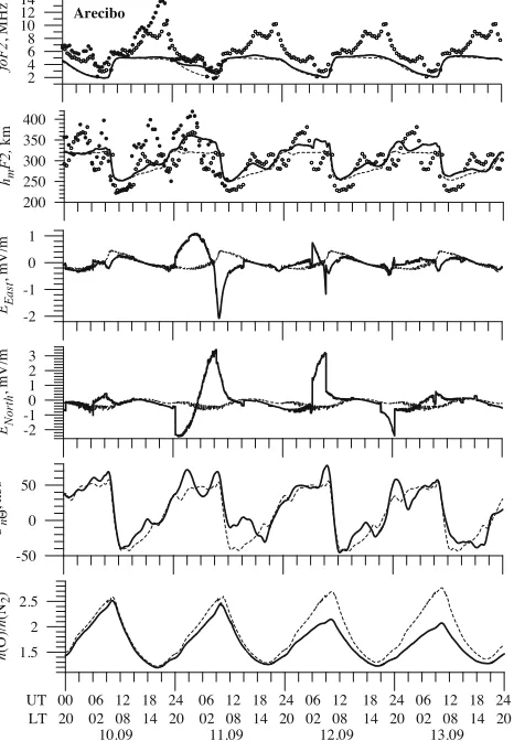
Figures 6 and 8 show the GSM TIP calculated behavior of
foF2andhmF2, the zonal and meridional components of the
electric field,EEastandENorth, the meridional component of
the thermospheric wind velocity,Un, and then(O)/n(N2)
ratio at a height of 300 km for Millstone Hill and Arecibo locations, respectively. The two top plots show the foF2
andhmF2variations from Millstone Hill and Arecibo ISRs
observation for the quiet and disturbed conditions.
The negative afternoon and evening disturbances in foF2
observa-Fig. 6. The behavior of: foF2,hmF2,EEast,ENorth,Unandn(O)/n(N2)
at height of 300 km above Millstone Hill. Dotted and thick lines—GSM TIP model results, light and dark circles—ISR data for quiet and storm conditions, respectively.
Fig. 7. The behavior of:EEast,ENorthandUnat height of 300 km above
station Millstone Hill. Dotted and solid lines—ISR data for quiet and storm conditions, respectively.
tions during the entire considered period except the positive disturbances in the afternoon on September 10. The sign of these disturbances is in agreement with the GSM TIP calculations; however, the calculated positive and negative disturbances in foF2 are much weaker than in the
obser-vations. IRI-2000 is well reproducing the negative foF2
Fig. 8. Same as Fig. 6, but above Arecibo.
disturbances above Millstone Hill (see Fig. 3) but not the positive disturbances.
The positive disturbances are caused by the meridional component of the thermospheric wind. The same conclu-sion has been made by Lu et al. (2008) and Klimenko
et al.(2011) in the modeling study of the positive phase of the September 10, 2005 ionospheric storm. The GSM TIP reduction of then(O)/n(N2)ratio above Millstone Hill
should lead to the decrease in the electron density. The re-sulting effect is defined by the combined action of the ther-mospheric wind and the neutral atmosphere composition. According to GSM TIP, the contribution of both compo-nents of the electric field to this positive disturbance is in-significant. At the same time, the Millstone Hill ISR obser-vations (Fig. 7) show the additional eastward and northward components of electric field, which in the given situation should lead to the positive effect in foF2. The GSM TIP
calculated positive disturbances in foF2 on September 11
and 12 from 06:00 to 09:00 UT are associated with the ac-tion of the addiac-tional eastward electric field, whereas the negative disturbances in foF2during September 11–13 are
associated with the strong reduction of then(O)/n(N2)
ra-tio.
According to both the GSM TIP calculations and the observations, the positive disturbances inhmF2have three
as-sociated with the additional eastward electric field. The additional equatorward wind amplifies the electric field ef-fect according to the observations. In GSM TIP the day time peak is associated with the increase of the equatorward wind, whereas the observations show the joint contribution of the additional eastward electric field and the equatorward wind. In GSM TIP the evening peak inhmF2is associated
with the effect of the additional equatorward wind which is reduced by the westward electric field.
Only the positive disturbances in foF2 and hmF2 on
September 10 were observed above Arecibo. GSM TIP also shows only the positive disturbances, but the IRI model pre-dicts only the negative disturbances. The afternoon posi-tive disturbances in foF2are associated with the additional
equatorward thermospheric wind, and the nighttime distur-bances are due to the joint action of the equatorward ther-mospheric wind and both components of the electric field. The reduction of then(O)/n(N2)ratio decreases these
pos-itive disturbances. According to GSM TIP the pospos-itive dis-turbances inhmF2 have three peaks: pre-sunrise, daytime,
and nighttime. The pre-sunrise and nighttime peaks inhmF2
are associated with the joint action of the additional east-ward electric field and the additional equatoreast-ward thermo-spheric wind. The day time peak is associated with increase of the equatorward thermospheric wind.
5.
Discussion
We have compared the GSM TIP calculations, the IRI-2000 predictions, and the observations at multiple locations. Figures 3–7 demonstrate that the IRI-2000 predicts the neg-ative disturbances in foF2 in good agreement with the
ob-servations. The exceptions are the observed positive dis-turbances in foF2 at Yakutsk, Irkutsk, Millstone Hill and
Arecibo. Thus, the main discrepancy between IRI-2000 and the observations is the absence of positive foF2
dis-turbances during the considered geomagnetic storms. Mir´o Amaranteet al.(2007) and Buresovaet al.(2010) show that the empirical storm-time ionospheric correction model captures more effectively the negative phases, while electron density enhancement during storms and the transi-tion between the different storm phases is reproduced with less accuracy. This model is not able to reproduce correctly the storm-induced rapid changes in the daily course of foF2,
i.e., the initial rapid positive ionospheric response to the storm onset (Buresovaet al., 2010). This is probably due to the insufficient number of observational data used in the development of the empirical storm-time ionospheric cor-rection model. It is likely that the update of this model with increased volume of observational data would improve its performance.
The comparison of the GSM TIP calculations and the ob-servations has revealed both the qualitative agreement and the quantitative disagreement. As suggested in Klimenko
et al. (2011), the possible reasons of the differences be-tween the GSM TIP calculations and the observations are the following: the coarse temporal resolution of the model input parameters (e.g., the three-hourKp-index), the use of
the dipole approach of geomagnetic field in the GSM TIP model, and the absence of solar flare effects in the model.
The prompt penetration electric fields from high latitudes
to the equator occurs due to the failure of shielding con-ditions of magnetospheric convection electric field by R2 FAC. Vasyl´ı¨unas (1970) has predicted a∼30 min delay of the shielding effect with respect to the development of the magnetospheric convection electric field. This delay leads to the penetration to the low latitudes of magnetospheric convection electric field at the increasing geomagnetic ac-tivity (Kikuchiet al., 2010), and Alfven layer electric field (overshielding effects) at the decreasing geomagnetic activ-ity (Kikuchi et al., 2010). The dependence of the model input parameters on the 3-hourKp-index allows correct
de-scription of the prompt penetration electric field or over-shielding only in the first 30 min after each change inKp
-index.
The use of the dipole approach in the GSM TIP model does not allow consideration of the distortions of the Earth’s magnetic field during geomagnetic storms. Tsyganenkoet al.(2003) pointed out that in any particle simulation of the inner magnetospheric dynamics during major storms, the use a dipolar or quasi-dipolar magnetic field model is in-adequate even at L ∼ 3–4. The magnetic field should be obtained either using a more realistic empirical model or by means of a fully self-consistent code, based on global parti-cle distributions and externally driven boundary conditions. This approach was used by Liet al.(2011) in a study of the superdense plasma sheet formation during storm-time. At the present stage of GSM TIP model development the use of a realistic geomagnetic field represents a difficult prob-lem which requires the development of an absolutely new model.
Despite the marked imperfections in the present problem statement, we have obtained a qualitative agreement (the disturbances with the same sign) with the observations and confirmed the conclusions about the main formation mech-anisms of ionospheric disturbances during the September 10, 2005 storm based on model calculations of Lu et al.
(2008). The GSM TIP calculations of the ionospheric ef-fects of the geomagnetic storm sequence show that the pos-itive ionospheric disturbances in foF2are mainly caused by
the equatorward thermospheric wind and the eastward com-ponent of the electric field. This positive effect is reduced by the neutral atmosphere composition change, which is the main mechanism of the negative disturbance formation. The other mechanism is the westward electric field and the poleward thermospheric wind.
6.
Conclusion
We have presented the modeling of the ionospheric ef-fects of September 9–14, 2005 geomagnetic storm and the comparison of the GSM TIP results and IRI-2000 predic-tions with the ionosonde and incoherent scatter radar ob-servations at Yakutsk, Irkutsk, Millstone Hill, and Arecibo. The main conclusions are the following.
1. The IRI-2000 model does not reproduce the positive storm time disturbances observed in the mid-latitude
in turn, strongly underestimates the observed positive phase of the ionospheric storm.
2. The GSM TIP disturbances are of the same sign as the ionosonde and ISR observations. The differences be-tween storm and quiet time are always smaller in the GSM TIP model than in the observational data. The largest discrepancies occurred at Irkutsk during day-time on September 11, 2005. We suggest that the causes of the differences between model calculations and data were the coarse (3-hour) resolution of the model drivers, the dipole approximation of geomag-netic field in GSM TIP, and also the possible effects of solar flares which are not included in GSM TIP calcu-lations.
3. The analysis of the observations and GSM TIP calcu-lations has shown that the positive ionospheric storm is mainly caused by the equatorward meridional ther-mospheric wind, and can be further enhanced by the eastward component of electric field. This positive ef-fect is reduced by the change of the neutral atmosphere composition which is the main formation mechanism of the negative disturbances in foF2.
Acknowledgments. The authors acknowledge the Irkutsk and Yakutsk digisonde teams and Arecibo and Millstone Hill ISR teams for processing the data and making the experimental data available. We express our gratitude to Prof. Bodo Reinisch for his help in evaluating this paper. These investigations were carried out with the financial support of the Russian Foundation for Basic Research (RFBR)—Grant No. 08-05-00274.
References
Balan, N., K. Shiokawa, Y. Otsuka, S. Watanabe, and G. J. Bai-ley, Super plasma fountain and equatorial ionization anomaly dur-ing penetration electric field, J. Geophys. Res., 114, A03310, doi:10.1029/2008JA013768, 2009.
Balan, N., K. Shiokawa, Y. Otsuka, T. Kikuchi, D. Vijaya Lekshmi, S. Kawamura, M. Yamamoto, and G. J. Bailey, A physical mechanism of positive ionospheric storms at low latitudes and midlatitudes,J. Geo-phys. Res.,115, A02304, doi:10.1029/2009JA014515, 2010.
Bilitza, D., International Reference Ionosphere 2000,Radio Sci.,36, 261– 275, 2001.
Bilitza, D., International Reference Ionosphere 2000: Examples of im-provements and new features,Adv. Space Res.,31, 757–767, 2003. Buonsanto, M. J., Ionospheric storms—a review,Space Sci. Rev.,88, 563–
601, 1999.
Buresova, D., L.-A. McKinnell, T. Sindelarova, and B. A. De La Morena, Evaluation of the STORM model storm-time corrections for middle latitude,Adv. Space Res.,46, 1039–1046, 2010.
Feshchenko, E. Yu. and Yu. P. Maltsev, Relations of the polar cap voltage to the geophysical activity, Proc. XXVI Annual Seminar “Physics of Auroral Phenomena”, pp. 59–61, February 25–28, 2003, Apatity, PGI KSC RAS, 2003.
Forbes, J. M., Dynamics of the thermosphere,J. Meteor. Soc. Jpn.,85B, 193–213, 2007.
Iijima, T. and T. A. Potemra, Field-aligned currents in the dayside cusp observed by triad,J. Geophys. Res.,81, 5971–5979, 1976.
Khmyrov, G. M., I. A. Galkin, A. V. Kozlov, B. W. Reinisch, J. McElroy, and C. Dozois, Exploring digisonde ionogram data with SAO-X and DIDBase,Radio Sounding and Plasma Physics, AIP Conf. Proc.,974, 175–185, 2008.
Kikuchi, T., K. K. Hasimoto, and K. Nozaki, Penetration of magneto-spheric electric fields to the equator during a geomagnetic storm, J. Geophys. Res.,113, doi:10.1029/2007JA012628, 2008.
Kikuchi, T., Y. Ebihara, K. K. Hashimoto, R. Kataoka, T. Hori, S. Watari, and N. Nishitani, Penetration of the convection and overshield-ing electric fields to the equatorial ionosphere durovershield-ing a quasiperiodic DP 2 geomagnetic fluctuation event,J. Geophys. Res.,115, A05209, doi:10.1029/2008JA013948, 2010.
Klimenko, M. V. and V. V. Klimenko, Numerical simulation effects of magnetospheric convection, particle precipitation and field aligned cur-rents of the second region during sequence of geomagnetic storms September 9–14, 2005,KSTU News, Kaliningrad, KSTU,16, 220–228, 2009 (in Russian).
Klimenko, M. V., V. V. Klimenko, and V. V. Bryukhanov, Numerical sim-ulation of the electric field and zonal current in the Earth’s ionosphere: The dynamo field and equatorial electrojet,Geomagn. Aeron.,46, 457– 466, 2006.
Klimenko, M. V., V. V. Klimenko, and V. V. Bryukhanov, Numerical mod-eling of the equatorial electrojet UT-variation on the basis of the model GSM TIP,Adv. Radio Sci.,5, 385–392, 2007.
Klimenko, M. V., V. V. Klimenko, K. G. Ratovsky, and L. P. Goncharenko, Ionospheric effects of geomagnetic storm sequence on September 9–14, 2005,Geomagn. Aeron.,51(3), 2011 (in print).
Klimenko, V. V. and A. A. Namgaladze, Ionospheric effects of meridional electric fields, inIonosphere Variations During Magnetospheric Distur-bances, Moscow, Nauka, 3–10, 1980 (in Russian).
Li, W., J. Raeder, M. F. Thomsen, and B. Lavraud, The formation of super-dense plasma sheet in association with the IMF turning from northward to southward,J. Geophys. Res.,116, doi:10.1029, 2011 (in print). Lu, G., L. P. Goncharenko, A. D. Richmond, R. G. Roble, and N. Aponte,
A dayside ionospheric positive storm phase driven by neutral winds,J. Geophys. Res.,113, doi:10.1029/2007JA012895, 2008.
Maruyama, N., S. Watanabe, and T. J. Fuller-Rowell, Dynamic and ener-getic coupling in the equatorial ionosphere and thermosphere,J. Geo-phys. Res.,108(A11), 1396, doi:10.1029/2002JA009599, 2003. Maruyama, N., A. D. Richmond, T. J. Fuller-Rowell, M. V. Codrescu,
S. Sazykin, F. R. Toffoletto, R. W. Spiro, and G. H. Millward, In-teraction between direct penetration and disturbance dynamo electric fields in the storm-time equatorial ionosphere,Geophys. Res. Lett.,32, doi:10.1029/2005GL023 763, 2005.
Mayr, H. G. and H. Volland, Magnetic storm characteristics of the thermo-sphere,J. Geophys. Res.,78, 2251–2264, 1973.
Mir´o Amarante, G., M. Cueto Santamar´ıa, K. Alazo, and S. M. Radicella, Validation of the STORM model used in IRI with ionosonde data,Adv. Space Res.,39, 681–686, 2007.
Namgaladze, A. A., Yu. N. Korenkov, V. V. Klimenko, I. V. Karpov, F. S. Bessarab, V. A. Surotkin, T. A. Glushenko, and N. M. Naumova, Global model of the thermosphere-ionosphere-protonosphere system,
Pure Appl. Geophys.,127, 219–254, 1988.
Namgaladze, A. A., Yu. N. Korenkov, V. V. Klimenko, I. V. Karpov, V. A. Surotkin, and N. M. Naumova, Numerical modelling of the thermosphere-ionosphere-protonosphere system,J. Atmos. Terr. Phys., 53, 1113–1124, 1991.
Reinisch, B. W. and I. A. Galkin, Global Ionospheric Radio Observatory (GIRO),Earth Planets Space,63(4), 377–381, 2011.
Rishbeth, H. and K. Garriott,Introduction to Ionospheric Physics, Aca-demic Press, New York, 1969.
Schunk, R. W., Response of the ionosphere-thermosphere system to mag-netospheric forcing,Adv. Space Res.,10(6), 133–142, 1990.
Sojka, J. J., R. W. Schunk, and W. F. Denig, Ionospheric response to the sustained high geomagnetic activity during the March ’89 great storm,
J. Geophys. Res.,99, 21341–21352, 1994.
Tsyganenko, N. A., H. J. Singer, and J. C. Kasper, Storm-time distortion of the inner magnetosphere: How severe can it get?,J. Geophys. Res., 108(A5), 1209, doi:10.1029/2002JA009808, 2003.
Vasyl´ı¨unas, V. M., Mathematical models of magnetosphere convection and its coupling to the ionosphere, inParticles and Fields in the Magneto-sphere, edited by McCormac, B. M., pp. 60–71, D. Reidel, Dordrecht, 1970.