DATA DRIVEN SOLUTIONS AND DISCOVERIES IN MECHANICS USING PHYSICS INFORMED NEURAL NETWORK

(1)

DATA DRIVEN SOLUTIONS AND DISCOVERIES IN MECHANICS

USING PHYSICS INFORMED NEURAL NETWORK∗

QI ZHANG†, YILIN CHEN †, AND ZIYI YANG‡

Abstract. Deep learning has achieved remarkable success in diverse computer science appli-cations, however, its use in other traditional engineering fields has emerged only recently. In this project, we solved several mechanics problems governed by differential equations, using physics in-formed neural networks (PINN). The PINN embeds the differential equations into the loss of the neural network using automatic differentiation. We present our developments in the context of solv-ing two main classes of problems: data-driven solutions and data-driven discoveries, and we compare the results with either analytical solutions or numerical solutions using the finite element method. The remarkable achievements of the PINN model shown in this report suggest the bright prospect of the physics-informed surrogate models that are fully differentiable with respect to all input co-ordinates and free parameters. More broadly, this study shows that PINN provides an attractive alternative to solve traditional engineering problems.

Key words. Conservation laws, Data inference, Data discovery, Dimensionless form, PINN

1. Introduction. It is well-known that many mechanics phenomenons are gov-erned by conservation laws which can be converted to differential equations for most of the applications. Solving these differential equations and obtaining parameter estimations from given observations are always intriguing topics, and significant re-search has been done to develop many advanced (semi-)analytical or numerical algo-rithms. While in the last decade, machine learning especially neural networks have yielded revolutionary results across diverse disciplines, including image and pattern recognition, natural language processing, genomics, and material constitutive model-ing [15,23,26,34], among which a fair amount of research has also been done related to differential equations [1,9,12,13,17–19,22,24,25,27–33,35,36,38], owing to the dra-matic increase in the computing resources. Therefore, it will be interesting to adopt neural networks as an important alternative to traditional mathematical methods to approximate the solutions to differential equations through iterative update of the network weights and biases.

2. Related work. Early researches that use neural network in scientific com-puting could date back to [12,22], in which a single hidden layer neural network is adopted

(2.1) N = ˜u+

H X

i=1 viσi



 n X

j=1

wijxj+ui 

 ,

where N is the network output which is assumed to be a scalar for illustration pur-poses,H is the width of the hidden layer, andnis the dimension of the input vector x∈Rn, wij andvi are called weights while ui and ˜uare always denoted as the

bi-ases,σi(·) is called activation function. More recently, the development of automatic

differentiation [2] has led to emerging literature on the use of deep neural networks to solve differential equations [17,33,38,39] even in complex geometries, and Berg

∗_{Stanford CS229 project final report, category of physical sciences}

†_{Department of Civil and Environmental Engineering,} _{Stanford University,} _{CA 94305}

([email protected],[email protected]).

‡_{Department of Mechanical Engineering, Stanford University, CA 94305 ([email protected]).}

1

(2)

et al. [3] provides details of this back propagation algorithm for advection and diffu-sion equations. Unlike traditional machine learning methods, deep neural networks sometimes can overcome the curse of dimensionality [17]. In the work done by Raissi et al [30–32], they named such strong form approach for differential equation as the physics-informed neural network (PINN) for the first time. Today, the PINN becomes more and more popular in many engineering fields such as hydrogeology [7,18,35], geomechanics [19], cardiovascular system [21] and so on. One attractive feature of PINN is that it is fully differentiable with respect to all the input coordinates and free parameters, in other words, the trial solution (via the trained PINN) represents a smooth approximation that can be evaluated and differentiated continuously on the domain [9]. Another important feature of PINN is that it can be used to solve inverse (data discovery) problems [16] with minimum change of the code from the forward problems [24].

It is also worth to mention that there are also other machine learning methods that didn’t rely on the neural network to solve differential equations [28,29], but in this report, we will focus on the PINN.

3. Methods. In this section, we will give a very brief overview of PINN in order to demonstrate how the loss functionLis defined in such context. We refer interested readers to look at [32] for more details. Consider a system of differential equations defined on the domain Ω with boundary∂Ω:

(3.1) D(u(x)) =0 x∈Ω,

(3.2) B(u(x)) =0 x∈∂Ω,

where u is the unknown solution vector, D denotes the abstract (non-linear) differ-ential operator (e.g., ∂/∂x, u◦∂/∂x,x◦∂/∂x, higher order derivatives, non-linear functions ofuorx, their combinations,etc.), and the operatorBexpresses arbitrary boundary conditions (e.g., Dirichlet, Neumann, Robin,etc.) associated with the prob-lem. Note here for time-dependent problems, we consider t as a special component of x, i.e., the Ω contains the temporal domain. The initial condition can be sim-ply treated as a special type of Dirichlet boundary condition on the spatio-temporal domain [24].

Now we construct a neural network with L layers, or L−1 hidden layers to approximate u(x), the input to neural network is x, and we will denote the output of the neural network as ˆu(x;θ) (we want ˆu(x;θ) ≈ u(x)), where θ represents the collection of weight matrixW[l] _∈_Rnl×nl−1 _{and bias vector} _b[l] _∈ _Rnl _{for each} layer l with nl neurons. In the inverse or data discovery problems, there are some

unknown parametersγ in the original differential equations, thus we will rewrite our approximation as ˆu(x;θ, γ). Now we can define the physics-informed lossL as

(3.3) L(θ, γ) =wfLf(θ, γ) +wbLb(θ, γ) +wdLd(θ, γ),

wherewf is the weight for the loss due to mismatch with the governing equations

(3.4) Lf(θ, γ) =

1 |Γf|

X

x∈Γf⊂Ω

kD( ˆu(x;θ, γ))k2₂ ,

andwb is the weight for the loss due to mismatch with the boundary conditions

(3.5) Lb(θ, γ) =

1 |Γb|

X

x∈Γb⊂∂Ω

(3)

and wd is the weight for the loss due to mismatch with the given data observations

u∗(x)

(3.6) Ld(θ, γ) =

1 |Γd|

X

x∈Γd⊂Ω

kuˆ(x;θ, γ)−u∗(x)k2₂ .

In practice, Γf and Γb are always known as the set of locations of the “residual”

points, and Γd is known as the set of measurement locations. We then optimizeθand

γ together, and our solution is

(3.7) θ∗, γ∗= argmin

θ,γ

L(θ, γ).

Above process is approximately summarized in Fig.1. Due to the network architecture and incorporation of differential equations, the loss will be highly non-linear and also non-convex, thus we will need some gradient-based optimizers, such as steepest descent [4], Newton’s method [4], Adam [20], and L-BFGS (limited-memory quasi-Newton method) [5]. In this report, we will adopt purely Adam or Adam combined with L-BFGS optimizers (i.e., we first use Adam for a certain number of iterations, and then switch to L-BFGS until convergence).

Fig. 1.Two schematics of the physics-informed neural network (PINN) [24,25].

For estimation of the test error, we will evaluate the lossLf on a given test set

Γtest ⊂Ω. In addition, if the true solution is available, we will also calculate the mean square error (similar to the form ofLd) on the same test set.

(4)

4. Experiments, results and discussions.

4.1. One dimensional consolidation problem. In soil mechanics, one of the most important processes is the consolidation process, while under some specific as-sumptions made by Prof. Terzaghi and Prof. Biot [6,8,37], we can mathematically quantify this process as a one dimensional diffusion problem [14] with specific bound-ary conditions and initial conditions. Suppose our problem domain is 0 ≤ x ≤ L whereLcan be understood as the thickness of the aquifer that rests on a rigid imper-meable base, at timet= 0, surface loadp0 is applied on the top of the aquifer which will lead to an initial pore pressure fieldpu₌_γ

lp0att= 0+whereγlis called loading

efficiency [37]. As time goes on, the pressure p will gradually decrease due to the effect of the drainage boundary atx= 0, and it satisfies following partial differential equation

(4.1) ∂ p

∂t −c ∂2_p ∂x2 = 0,

with boundary conditions p = 0 at x = 0 and ∂p/∂x = 0 at x = L. The initial condition is just p = pu as mentioned before. In above Eq. (4.1), the c is called generalized consolidation coefficient [11] which has the unit of length squared divided by time.

However, the order of magnitudes of different physical quantities x (order of meters), t (order of months) and p (order of kPa) could cast great difficulty on the training of the neural networks [21], and to overcome this problem, we employ a non-dimensionalization technique with the purpose of scaling the input and the output of the neural network in proper scales (e.g., O(1)). As a result, we will introduce characteristic values for x and p, and for this problem an obvious choice would be characteristic length L and characteristic pressure pu_{. At this point we define the} dimensionless quantities as

(4.2) xˆ= x

L pˆ= p pu.

For the timet, the dimensionless time ˆt is given as

(4.3) ˆt= ct

L2.

Now all the variables take values withO(1) magnitude and we will rewrite Eq. (4.1) using dimensionless variables, the result is shown as follows

(4.4)

∂pˆ ∂ˆt −

∂2_p_ˆ

∂xˆ2 = 0 0<x <ˆ 1 ˆt >0 ˆ

p= 0 xˆ= 0 ˆt≥0 ∂pˆ

∂xˆ = 0 xˆ= 1 ˆt >0 ˆ

p= 1 0<xˆ≤1 ˆt= 0.

The analytical solution for Eq. (4.4) is given as

(4.5) pˆ=

∞ X

m=1,3,5,7,...

4 mπsin

_mπ_x_ˆ

2

e−m

2_π2 ˆt

(5)

For the PINN hyper-parameters, we assume ˆtmax = 0.5, and we draw 500, 250, 125 “residual” points randomly from (0,1)× 0,ˆtmax, boundary of ˆxand boundary of ˆt respectively to form Γf and Γb. The test set Γtest will have 10011 points. The

loss weights are assigned as wf = wb = 1/4 (wd is not used in this problem). For

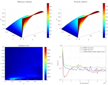
the architecture of the neural network, it will contain 5 hidden layers with 50 neurons each, and we will use hyperbolic tangent tanh as our activation function in hidden layers, the output activation will be linear activation but we will multiply the network output with ˆxas our final output, because in this way our output will automatically satisfy the second expression in Eq. (4.4). For the optimization procedure, we will run Adam for 50000 epochs with learning rate 0.001 and then run L-BFGS until convergence. For the network initialization, we will use the Glorot normal initializer. The convergence history, reference solution, PINN solution, and the absolute error is shown in the Fig. 2, from which we can see a perfect match is achieved, and the locations with highest error is close to the origin due to sharp gradient. Note in Fig.2, we have enforced all the output values are between 0 and 1, and initial condition is strictly satisfied.

Fig. 2.PINN training results for the one dimensional consolidation problem.

4.2. Steady state heat conduction problem. Our second example is a time-independent problem on 2D. In the steady state heat transfer problem with constant heat conduction coefficient, constant heat source and constant boundary temperature (Dirichlet boundary condition), the T will satisfy Poisson’s equation [14]. Without loss of generality and to avoid the scaling differences, we will solve following PDE on

(6)

Ω = [−1,1]×[−1,1]

(4.6) ∂

2_T

∂x2 + ∂2_T

∂y2 + 1 = 0 −1< x <1 −1< y <1,

(4.7) T = 0 (x, y)∈∂Ω.

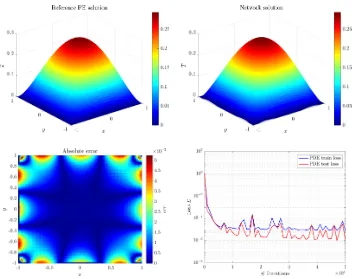
Even though the analytical solution for this problem doesn’t exist, the finite element solution with high accuracy is available indeal.II finite element library tutorial 3, thus it will be interesting to compare these two numerical solutions.

For the PINN hyper-parameters, we choose 1500 and 500 random points to form Γf and Γb, respectively. The test set Γtestwill have 10000 points. The loss weights are assigned aswf =wb = 1/2 (wd is not used in this problem). For the architecture of

the neural network, it will contain 4 hidden layers with 50 neurons each, and we will not apply any transform for the network output. The learning rate for this problem is 0.0005. For the network initialization, we will use the Glorot uniform initializer. The remaining settings are the same as the first example.

The training results are shown in the Fig. 3, where the two numerical solutions are consistent with each other. Note in Fig.3, we have enforced all the output values are larger than 0. The largest absolute error happens near the Dirichlet boundary because Eq. (4.7) is not regarded as a hard constrain in the construction of the loss L. A feasible way to handle this problem would be to introduce a smoothdistance function ˆd(x) that gives the distance forx∈Ω to∂Ω [3], and then we multiply ˆdwith the original network output to get our new improved output, which will automatically satisfy Eq. (4.7).

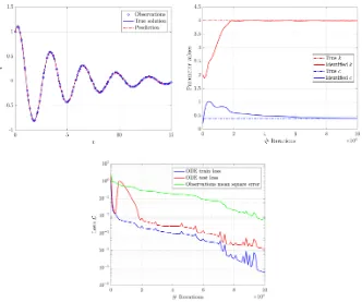
4.3. Inverse problem for simple structural dynamic system. The last example comes from the dynamic response of the single degree of freedom system [10] and we want to use this example to illustrate the capability of PINN in the inverse modeling or data discovery process. In structural dynamics, the free vibration equation with viscous damping for single mass point is obtained through D’Alembert principle [10]

(4.8) md

2_u

dt2 +c du

dt +ku= 0 t >0

with u(0) = u0 and ˙u(0) = v0. In above equation, m > 0 is the mass, c > 0 is the damping coefficient, k >0 is the stiffness,uis the displacement,u0 is the initial displacement and v0 is the initial velocity. The analytical solution to this ODE is given as

(4.9) u(t) = e−ξωnt

u0cos (ωDt) +

v0+ξωnu0 ωD

sin (ωDt)

,

where ωn = p

k/m is known as the natural frequency, ξ =c/(2mωn) is known as

the damping ratio,ωD=ωn p

1−ξ2_{. In this problem, we will assume}_{ξ <}_{1 which is} known as the underdamped system.

(7)

Fig. 3.PINN training results for the steady state heat conduction problem.

10000 points to form Γtest. The loss weights are assigned aswf =wb =wd = 1/4.

For the architecture of the neural network, it will contain 3 hidden layers with 32 neurons each, and we will not apply any transform for the network output. For the optimization procedure, we will only run Adam for 100000 epochs with learning rate 0.0005. For the network initialization, we will use the Glorot uniform initializer.

The evolution trajectories ofc andkare presented in Fig. 4, with final values of ¯

k= 3.9933197 and ¯c= 0.40125215, which agree with their true values.

5. Conclusions. In this project, we have adopted PINN, a new class of univer-sal function approximators that is capable of encoding any underlying conservation laws which can be described by differential equations. Compared to the traditional numerical methods, PINN employs automatic differentiation to handle differential op-erators, and thus are mesh-free. We use PINN as a data driven algorithm for inferring solutions and parameter identifications of differential equations. A series of promising results for a diverse collection of problems in mechanics are presented and discussed, which opens the path for endowing deep learning with the powerful capacity of math-ematical physics to model the world around us. We hope this project could benefit future practitioners across a wide range of scientific domains who want to incorporate deep learning methods in modeling physics-related problems.

For the future work, it is worth to try a group of coupled differential equations such as Eqs. (5.1)(5.2) in poromechanics [40] to see the PINN’s performance, and develop some training points selection strategy similar to the adaptive re-meshing in

(8)

Fig. 4. PINN training results for the parameter identification problem, the identified values

converge to the true values during the training process.

the mesh-based methods to achieve better accuracy.

(5.1) 1

M ∂ p

∂t − k µf

∇2p+α∂∇ ·u ∂t = 0,

(5.2) G∇2_u₊ G

1−2ν∇(∇ ·u)−α∇p+ρbg=0.

(9)

REFERENCES

[1] Y. Bar-Sinai, S. Hoyer, J. Hickey, and M. P. Brenner,Learning data-driven discretizations for partial differential equations, Proceedings of the National Academy of Sciences, 116 (2019).

[2] A. G. Baydin, B. A. Pearlmutter, A. A. Radul, and J. M. Siskind,Automatic differ-entiation in machine learning: a survey, The Journal of Machine Learning Research, 18 (2017).

[3] J. Berg and K. Nystr¨om,A unified deep artificial neural network approach to partial differ-ential equations in complex geometries, Neurocomputing, 317 (2018).

[4] S. Boyd and L. Vandenberghe,Convex optimization, Cambridge university press, 2004. [5] R. H. Byrd, P. Lu, J. Nocedal, and C. Zhu,A limited memory algorithm for bound

con-strained optimization, SIAM Journal on scientific computing, 16 (1995), pp. 1190–1208. [6] N. Castelletto, J. A. White, and H. A. Tchelepi,Accuracy and convergence properties of

the fixed-stress iterative solution of two-way coupled poromechanics, International Journal for Numerical and Analytical Methods in Geomechanics, 39 (2015).

[7] X. Chen, J. Duan, and G. E. Karniadakis, Learning and meta-learning of sto-chastic advection-diffusion-reaction systems from sparse measurements, arXiv preprint arXiv:1910.09098, (2019).

[8] A. H. D. Cheng,Poroelasticity, Springer, 2016.

[9] M. Chiaramonte and M. Kiener,Solving differential equations using neural networks, CS229 Project, (2013).

[10] A. K. Chopra,Dynamics of structures: theory and applications to earthquake engineering, Prentice Hall, 1995.

[11] E. Detournay and A. H. D. Cheng,Fundamentals of poroelasticity, in Analysis and design methods, Elsevier, 1993, pp. 113–171.

[12] M. W. M. G. Dissanayake and N. Phan-Thien,Neural-network-based approximations for solving partial differential equations, Communications in Numerical Methods in Engineer-ing, 10 (1994), pp. 195–201.

[13] T. Dockhorn,A discussion on solving partial differential equations using neural networks, arXiv preprint arXiv:1904.07200, (2019).

[14] L. C. Evans,Partial differential equations, American Mathematical Society, 2010.

[15] J. Ghaboussi, J. H. Garrett Jr, and X. Wu,Knowledge-based modeling of material behavior

with neural networks, Journal of engineering mechanics, 117 (1991).

[16] E. Haghighat, M. Raissi, A. Moure, H. Gomez, and R. Juanes,A deep learning frame-work for solution and discovery in solid mechanics: linear elasticity, arXiv preprint arXiv:2003.02751, (2020).

[17] J. Han, A. Jentzen, and E. Weinan,Solving high-dimensional partial differential equations

using deep learning, Proceedings of the National Academy of Sciences, 115 (2018). [18] Q. He, D. Barajas-Solano, G. Tartakovsky, and A. M. Tartakovsky,Physics-informed

neural networks for multi-physics data assimilation with application to subsurface trans-port, Advances in Water Resources, (2020), p. 103610.

[19] T. Kadeethum, T. M. Jørgensen, and H. M. Nick,Physics-informed neural networks for

solving nonlinear diffusivity and biot’s equations, PloS one, 15 (2020), p. e0232683. [20] D. P. Kingma and J. Ba, Adam: A method for stochastic optimization, arXiv preprint

arXiv:1412.6980, (2014).

[21] G. Kissas, Y. Yang, E. Hwuang, W. R. Witschey, J. A. Detre, and P. Perdikaris,

Machine learning in cardiovascular flows modeling: Predicting arterial blood pressure from non-invasive 4d flow mri data using physics-informed neural networks, Computer Methods in Applied Mechanics and Engineering, 358 (2020).

[22] I. E. Lagaris, A. Likas, and D. I. Fotiadis,Artificial neural networks for solving ordinary and partial differential equations, IEEE transactions on neural networks, 9 (1998). [23] M. Lefik, D. P. Boso, and B. A. Schrefler,Artificial neural networks in numerical

model-ling of composites, Computer Methods in Applied Mechanics and Engineering, 198 (2009). [24] L. Lu, X. Meng, Z. Mao, and G. E. Karniadakis,DeepXDE: A deep learning library for

solving differential equations, arXiv preprint arXiv:1907.04502, (2019).

[25] X. Meng, Z. Li, D. Zhang, and G. E. Karniadakis,Ppinn: Parareal physics-informed neural network for time-dependent pdes, arXiv preprint arXiv:1909.10145, (2019).

[26] M. Mozaffar, R. Bostanabad, W. Chen, K. Ehmann, J. Cao, and M. A. Bessa,Deep learn-ing predicts path-dependent plasticity, Proceedings of the National Academy of Sciences, 116 (2019).

[27] M. Raissi,Deep hidden physics models: Deep learning of nonlinear partial differential

(10)

tions, The Journal of Machine Learning Research, 19 (2018), pp. 1–24.

[28] M. Raissi and G. E. Karniadakis,Hidden physics models: Machine learning of nonlinear

partial differential equations, Journal of Computational Physics, 357 (2018), pp. 125–141. [29] M. Raissi, P. Perdikaris, and G. E. Karniadakis,Machine learning of linear differential equations using gaussian processes, Journal of Computational Physics, 348 (2017), pp. 683– 693.

[30] M. Raissi, P. Perdikaris, and G. E. Karniadakis, Physics informed deep learning (part

i): data-driven solutions of nonlinear partial differential equations, arXiv preprint arXiv:1711.10561, (2017).

[31] M. Raissi, P. Perdikaris, and G. E. Karniadakis, Physics informed deep learning (part ii): data-driven discovery of nonlinear partial differential equations, arXiv preprint arXiv:1711.10566, (2017).

[32] M. Raissi, P. Perdikaris, and G. E. Karniadakis,Physics-informed neural networks: A deep learning framework for solving forward and inverse problems involving nonlinear partial differential equations, Journal of Computational Physics, 378 (2019), pp. 686–707. [33] J. Sirignano and K. Spiliopoulos,Dgm: A deep learning algorithm for solving partial

dif-ferential equations, Journal of Computational Physics, 375 (2018), pp. 1339–1364. [34] Y. Sun, W. Zeng, Y. Zhao, X. Zhang, Y. Shu, and Y. Zhou,Modeling constitutive

relation-ship of ti40 alloy using artificial neural network, Materials & Design, 32 (2011).

[35] A. Tartakovsky, C. O. Marrero, P. Perdikaris, G. Tartakovsky, and D. Barajas-Solano,Physics-informed deep neural networks for learning parameters and constitutive relationships in subsurface flow problems, Water Resources Research, 56 (2020).

[36] J. Tompson, K. Schlachter, P. Sprechmann, and K. Perlin,Accelerating eulerian fluid simulation with convolutional networks, in Proceedings of the 34th International Confer-ence on Machine Learning, 2017.

[37] H. F. Wang,Theory of linear poroelasticity with applications to geomechanics and hydrogeol-ogy, Princeton University Press, 2000.

[38] E. Weinan, J. Han, and A. Jentzen, Deep learning-based numerical methods for high-dimensional parabolic partial differential equations and backward stochastic differential equations, Communications in Mathematics and Statistics, 5 (2017), pp. 349–380. [39] E. Weinan and B. Yu,The deep ritz method: a deep learning-based numerical algorithm for

solving variational problems, Communications in Mathematics and Statistics, 6 (2018), pp. 1–12.