c
Owned by the authors, published by EDP Sciences, 2012
Complex modulus estimation respecting causality: Application to
viscoelastic bars
P. Collet
1, G. Gary
2, B. Lundberg
2,3, and D. Mohr
21Centre de Physique Th ´eorique CNRS UMR 7644, ´Ecole Polytechnique, 91128 Palaiseau, France
2Laboratoire de M ´ecanique des Solides, CNRS UMR 7649, ´Ecole Polytechnique, 91128 Palaiseau, France 3The ˚Angstr ¨om Laboratory, Uppsala University, Box 534, SE-751 21 Uppsala, Sweden
Abstract. The identification of linear visco-elasticity models mostly focuses on the real and imaginary parts of the Young’s modulus. Many methods have been proposed in the past to identify these material model parameters from experiments. However, when these parameters are determined independently, they are likely to violate the principle of causality. The present work presents a method that accounts for the constraints of causality and positivity of dissipation rate. The proposed method is based on a finite set ofnmeasured angular frequencies and complex moduli. It includes a noise reduction procedure and provides a rheological 2p+1)-parameter model withp<gn which corresponds to a specific configuration of pairs of springs and dashpots. The poles of the complex modulus on the positive imaginary frequency axis are determined bypparameters which are obtained as the common positive zeros of a special class of rational functions, while the remaining parameters are obtained from a least squares fit. The level of refinement of the rheological model, expressed byp, is not an assumed value but a result of the method. The method is applied to an impact test with a Nylon bar specimen. In this case, data at then=29 lowest resonance frequencies resulted in a rheological model with 14 parameters (p = 6). The validity of the method is checked through supplementary experimental results at low frequencies.
1 Introduction
Methods for estimation of the properties of viscoelas-tic materials have been proposed and used since long. Such methods, devoted to estimation of complex-valued frequency-dependent material parameters such as the com-plex modulus, generally produce data from which discrete values of the parameters can be obtained for a set of frequencies.
For the measurement of viscoelastic properties, ma-chines for dynamic mechanical analysis (DMA) are com-mercially available. A review of such machines can be found in [1]. Most methods make use of the vibration of a particular structure [2–5]. Wave propagation in bars has also been used to determine the viscoelastic properties of materials [6–12].
Often, it is not ensured that the real and imaginary parts of the complex modulus are consistent with the principle of causality. One way to achieve such consis-tency is to express them in terms of a rheological model constituted by linear springs and dashpots [5, 13]. An alternative way consists in making sure that the complex modulus is consistent with the Kramers-Kronig relations. Another fundamental constraint on the complex modulus comes from the second principle of thermodynamics: the dissipation per cycle must be positive for any harmonic load. Furthermore, the relaxation function, which is the inverse Fourier transform of the complex modulus, must be real. About these constraints, see, e.g. [14, 15]
In this paper we present a method for noise-corrected estimation of the complex modulus of a viscoelastic ma-terial, subject to the constraints of causality, positivity of dissipation and reality of relaxation function, given an experimental set of frequencies and corresponding values
of the complex modulus. The estimation method provides the structure, the number and type of elements (springs and dashpots) and the parameters of a rheological model for the complex modulus. It will be illustrated with experimental data obtained by impacting a Nylon bar specimen.
2 Estimation method
2.1 Theory
According to Boltzmann’s model of viscoelastic materials, and after Fourier transformation, the relation between stressσ(t) and strainε(t) is given by
ˆ
σ(ω)=E(ω) ˆε(ω),
whereE(ω) is the complex modulus andωis the angular frequency.
The complex modulus must satisfy the three con-straints of causality, positivity of the dissipation rate and reality of the relaxation function. The problem to be considered is that of finding a noise-corrected complex modulusE(ω), subject to these constraints, given a finite set of angular frequencies and corresponding complex moduli obtained experimentally.
The constraint of causality implies the Kramers-Kronig relations that connect the real and imaginary parts of the complex modulus. If either the real or the imaginary part can be estimated accurately at a sufficient number of frequencies, these relations can be used to estimate the other part. With the experimental method of this paper, results for the complex modulus are obtained only for a relatively small set of frequencies. Therefore, we adopt
imaginary parts of the complex modulus.
The constraints of causality and of positivity of the dissipation rate [14–17] are equivalent to requiring that the functionE(ω) be analytic in the lower half plane and that its imaginary part be positive on the positive real axis, respectively. The constraint of reality of the relaxation function is equivalent to the requirementE(−ω)=E(ω). Here we will use the stronger constraint of complete monotonicity of the relaxation function [17, 18]. This con-straint, which essentially means that the relaxation func-tion and its derivatives must be monotone, is satisfied by most rheological models [17]. To which extent it holds for a particular real material can be verified from experimental data.
The property of complete monotonicity of the relax-ation function implies that this function is the Laplace transform of a positive function (the Bernstein-Widder Theorem, see [17]). This means that the complex modulus E(ω) is the sum of a linear function and a Stieltjes transform. More precisely, there exist two parameters α0 > 0 and β0 ≥ 0 a functionh(s) ≥ 0, defined on the positive real axis such that
E(ω)=α0+iωβ0−
∞
0 h(s)
s+iωds. (1) Such functions (1) are analytic outside the positive imag-inary axis of the complex plane and they satisfy the three constraints. Thus, they are analytic in the lower half plane and therefore satisfy the constraint of causality; their imaginary part is positive on the positive real axis and therefore the constraint of positiveness of the dissipation rate holds. Finally, the constraint of reality of the relaxation function is satisfied asE(−ω)=E(ω).
In order to check whether experimental data are of the form of Eq. (1), in particular for the purpose of determining the constantsα0andβ0, and the functionh, it is convenient to apply the transformation f(z) = −E(izz) that has the representation
f(z)=β0+
g
(s)
s−zds, (2) with
g(s)=
α0−
∞
0 h(u)
u du
δ(s)+ h(s) s ,
whereδ(s) is a delta function at the origin, andg(s)=0 for s < 0. The function f(z) is analytic except on the positive real axis, and positive on the negative real axis.
The problem of finding a function f(z) with the rep-resentation (2) given its values for finitely many z was studied in detail by Krein and Nudelman [19]. Some of their results, when formulated for the complex modulus E(ω), are as follows. From the values E1,E2, . . . , En of
the functionE(ω) atnangular frequenciesω1,ω2, . . . ,ωn
one can form two matrices with elements M(1)j,k =iωE¯j−Ek
j+ωk =
β0+
∞
0
h(s) ds s−iωj
(s+iωk)
,
(3)
Mj,k =
ωj+ωk
= ωE(0) jωk +
∞ 0 h(s) s ds
s−iωj
(s+iωk)
. (4)
It can be verified that the matrix M(1) is positive semi-definite. The same properties hold forM(2)sinceE(0)>0. If one of the matricesM(1)orM(2) has a zero eigenvalue, the function E(ω) is completely determined and is a rational fraction (see [19] and below).
Assume now thatais an eigenvector corresponding to a zero eigenvalue ofM(1). Then, sinceM(1)a=0,we also havea,M(1)a=0, i.e.,
β0
n
k=1 ak 2 + ∞ 0 h(s) n
k=1 ak
s+iωk
2
ds=0.
Since both terms in the left member are non-negative, they must vanish. In particular, the function h(s) must be a linear combination pl=1γlδ(s−sl) with coefficients
γl ≥ 0 of delta functions δ(s−sl) at the positive zeros
s1, . . . ,sp (p<n) of the rational function n
k=1 ak
s+iωk
. (5)
For the complex modulus given by Eq. (1) this implies the model
E(ω)=α0+iωβ0−
l=p
l=1 γl
sl+iω
, (6)
whereα0>0 andβ0,γ1,γ2, . . . ,γpare non-negative.
The same considerations hold for the matrixM(2)and should lead to the same model. If b is an eigenvector corresponding to a zero eigenvalue ofM(2), we deduce as above that the function h(s) must also be a linear combi-nation with non-negative coefficients of delta functions at the positive zeros of the rational function
n
k=1 bk
s+iωk
. (7)
In particular, we only need to consider the common posi-tive zeros of the rational functions (5) and (7). Moreover, if there are several linearly independent eigenvectors corre-sponding to a zero eigenvalue, we get a set of positive zeros for each of them and should keep only the ones which are common.
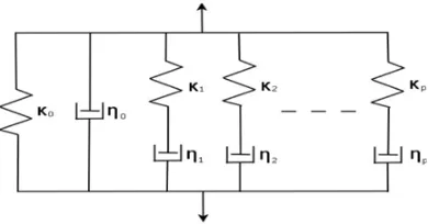
The model (6) for the complex modulus corresponds to the rheological model with 2 (p+1) parameters shown in Fig. 1.
The complex modulus represented by this model is
E(ω)=κ0+iωη0+
p
l=1 iωκl
κl/ηl+iω =κ0+
p
l=1
κl+iωη0−
p
l=1 κ2
l/ηl
κl/ηl+iω
Fig. 1.Rheological model with 2(p+1) parameters.
The p + 1 stiffnessesκ0,κ1, . . .κpof the springs and the
p +1 viscositiesη0,η1, . . .ηpof the dashpots are related
to the 2 (p+1) parameters andα0,β0,s1,s2, . . . ,sp,γ1, γ2, . . . ,γpof Eq. (6) by the relations
κ0 =α0−
p
l=1 γl
sl
, κl=
γl
sl
, η0=β0,
ηl=
γl
s2
l
, l=1, 2, . . . ..
2.2 Implementation
From experiments, we obtain a finite set of angular fre-quencies ω1, . . . , ωn and corresponding complex moduli
E1, . . .En. By use of these experimental data we form the
two matricesM(1)j,k andM(1)j,k given by the first equalities of Eqs. (3) and (4), respectively. These self-adjoint matrices are positive semi-definite if and only if all their eigenvalues are non-negative. However, experiments commonly result in some slightly negative eigenvalues. In the experimental part of this paper, for example, the modulus of the smallest negative eigenvalue is typically a few tenths of a percent of the largest positive eigenvalue. A likely explanation for such small violations of the positive semi-definiteness is experimental noise. As advocated in [20] for a sim-ilar problem, the effects of such noise can be reduced by searching the smallest possible corrections of angular frequencies and moduli which restore the non-negativeness of all eigenvalues and establishing noise-corrected sets ωcorr
1 , ..., ω corr
n andE1corr, . . . ,Ecorrn .
If at least one of the noise-corrected matricesM(1)corr andM(2)corr has a zero eigenvector, one forms the associ-ated rational fraction (5) or (7) and finds its positive zeros. This is repeated for the set of independent eigenvectors, if any, corresponding to zero eigenvalues of both matrices. Then one keeps the common positive zeros s1, . . . ,sp of
all these rational fractions and obtains the model given by Eq. (6). In this model theppositive parameterss1, . . . ,sp
are known, while α0 > 0, β0 ≥ 0 and the p non-negative parameters γ1, γ2, . . . , γp are identified by a
least square fit of the model to the noise-corrected data. In this way, the method provides the structure, the number of elements (springs and dashpots) and the parameters of the rheological model. Normally, the number 2(p+1) of elements is found to be relatively low.
The experimental set of angular frequencies and corre-sponding values of the complex modulus may be obtained
l x
0 a
Fig. 2.Impact test with a uniform viscoelastic bar specimen.
with a variety of methods, quasi-static as well as dynamic. In what follows they will be obtained by analysing the wave propagation in a Nylon bar specimen loaded through axial impact.
3 Impact test method
3.1 Theory
Here, discrete values of the complex modulus E(ω) = E(ω) + iE(ω) will be obtained from the resonances of an impacted uniform bar specimen with densityρand lengthlas shown in Fig. 2.
At one end, x = 0, the bar is impacted axially by a striker that separates from the bar after the generation of a compressive primary pulse in the bar. The other end of the bar, x = l, is free. The strain εb(t) = ε(b,t) is
recorded at a distanceafrom the free end andbfrom the impacted end (a + b = l). The primary pulse should be shorter than 2aso that there is no overlap in the measured strain of this pulse and the first pulse reflected from the free end. However, it should be much longer than the diameter of the bar so that approximate 1D conditions prevail (wavelengths much longer than the diameter of the bar [21].
In the frequency domain, the strain in the bar can be expressed as
ˆ
ε(x, ω)=A(ω)e−iξ(ω)x+B(ω)eiξ(ω)x, (9) where
ξ2(ω)=ρω2/E(ω), ξ(ω)=k(ω)−iα(ω) (10) Here, ˆε(x, ω) is the Fourier transform ofε(x,t), andA(ω) and B(ω) are complex amplitudes of waves travelling in the directions of increasing and decreasing x, respec-tively,k(ω) is the wave number andα(ω) is the damping coefficient.
In order to determine an expression for the recorded strain ˆε1
b(ω)= εˆ(b, ω) associated with the primary pulse
alone, the amplitudes A andB are first determined from Eq. (9) and the boundary conditions ˆε(0, ω)=εˆ0(ω) and B(ω) = 0 for a semi-infinite bar x ≥ 0, where ˆε0(ω) is the strain at the impacted end. With these amplitudes and x=binserted, Eq. (9) give
ˆ ε1
b(ω)=e−
iξb
ˆ
andl−b=ainserted, Eq. (9) gives ˆ
ε∞ b (ω)=
sin (ξa)
sin (ξl)εˆ0(ω). (12) Dividing the members of Eq. (12) by those of Eq. (11) eliminates the strain ˆε0(ω) at the impacted end which normally cannot be measured. The elimination of this strain makes the difference between the method used here and that used by Othman et al. [22]. Substitutingξfrom the second of Eqs. (10) into the result, one gets the ratio
ˆ ε∞
b (ω)/ˆε1b(ω) which gives εˆ∞b (ω)
2
=εˆ1b(ω)
2 e2αbsin
2(ka)+sinh2(αa)
sin2(kl)+sinh2(αl) . (13) Resonance occurs at the angular frequencies ω = ωm,
m =1, 2, . . . which correspond to the wave numbers, wavelengths and phase velocities
km=
mπ
l , λm= 2π km =
2l
m, cm= ωm
km =
ωml
mπ, (14) respectively.
It is assumed that within them:thresonance peakα= αmω/ωmcan be taken as directly proportional to angular
frequency and c(ω) = ω/k(ω) = cm can be taken as
constant. By use of the third of Eqs. (14) we then obtain the relationk(ω) = kmω/ωmbetween wave number and
angular frequency within the resonance peak. Inserting these expressions forα(ω) andk(ω) into Eq. (13) we get
εˆ∞b (ω)2=εˆ1b(ω)2 ×e2αmbω/ωmsin
2(k
maω/ωm)+sinh2(αmaω/ωm)
sin2(kmlω/ωm)+sinh2(αmlω/ωm)
m=1, 2, . . . (15)
within them:thresonance peak. In this relation, the spectra
εˆ∞b (ω)2andεˆ1b(ω)2can be determined experimentally. For each resonancem = 1,2, . . ., the resonance fre-quencyωmand damping coefficient αm can be estimated
by minimizing the difference between the resonance peaks represented by the left and right members of Eq. (15). From ωm andm, the complex modulusEm at each
reso-nance frequency can be finally obtained as
Em=ρ ω
m
ξm 2
, ξm=
mπ
l −iαm, m=1,2,
3.2 Experimental set-up and procedure
Impact tests were carried out with a Nylon bar speci-men of length 3045 mm, diameter 10.2 mm, and density 1149 kg/m. Two pairs of strain gauges, one axial and one circumferential, were located at a distance of 1731 mm from the free end and 1314 mm from the impacted end. In order to minimise the effects of friction, the bar was suspended horizontally by means of nine regularly spaced
Fig. 3.Recorded strain in the Nylon bar specimen. (a) Long-time
record of strain pulses.
Fig. 4.Primary strain pulse followed by strain pulses which have
undergone one and two free-end reflections.
strings with length 300 mm. With this arrangement, the period of oscillation of the system was about one second, which is much longer than the test duration. The striker had length 174 mm and the same diameter 10.2 mm and material as the bar, and its impact velocity was 3.7 m/s. The strain was recorded with 500 kHz sampling frequency, and the signal vanished completely before the end of the recording window.
Results were evaluated up to 8 kHz. With a phase velocity expected to be higher than 1500 m/s at this fre-quency, the shortest significant wave length was estimated to be greater than 0.19 m. This wave length is much larger than the diameter 0.01 m of the bar, which means that 3D effects can be neglected as assumed in Section 3.1.
4 Results and discussion
The estimation method presented provides a model for the complex modulus corresponding to that shown in Fig. 1, withp +1 pairs of springs and dashpots. Consequently,p represents the complexity of the material behaviour. It is not an assumed value but a result of the method.
The recorded strain is shown in Figs. 3 and 4. Figure 3 shows a long-time record, and Fig. 4 shows the primary compressive pulse followed by one tensile and one com-pressive pulse which have undergone one and two free-end reflections, respectively. As there is no significant overlap of these pulses, it was possible to compute the spectrum
εˆ1
b
2
in the right member of Eq. (30) from the measured primary pulse.
Fig. 5.Details of the spectrum. The thin and thick curves are based on the left and the right member of Eq. (30), respectively. (upper) 1st resonance peak (lower) 25th resonance peak.
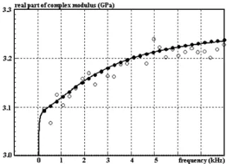
Fig. 6.Real part of the complex modulus versus frequency.
the resonance peaks determined from the left and right members of Eq. (30). For the material of the Nylon bar specimen tested, a rheological model with p = 6 was obtained forn=29.
For this model, the 14 parameters of Eq. (8), repre-senting the springs and dashpots in Fig. 1, are (l=0, 1, . . . ,6)κl = 2070, 1030, 2.96, 14.1, 28.5, 97.6, 24.8 MPa
ηl=0.663, 10800, 1.12, 2.48, 2.58, 5.02, 0.504 kPas.
Figures 6 and 7 show the frequency dependency of the real and imaginary parts of the complex modulus, viz., discrete experimental results, discrete noise-corrected results, and continuous results for the rheological model given by Eqs. (6) and (8) with the above sets of parameters. From the discrete experimental results for the phase velocity and the damping coefficient, the discrete exper-imental results for the complex modulus (open circles) were obtained as described in Section 3. The correspond-ing discrete noise-corrected results (filled circles) and the continuous results for the rheological model obtained as described in Section 2.1 are shown in the same figures.
While the experimental results are scattered due to noise, there is close agreement between the noise-corrected results and the smooth curves representing the rheolog-ical model. This indicates that the noise-correction was effective and that the rheological model obtained with
Fig. 7.Imaginary part of the complex modulus versus frequency.
p=6 provides an adequate representation of the complex modulus in the frequency range of the test.
At low frequencies, much below the range of the test, the rheological model cannot be expected to give a quantitatively accurate representation of the complex modulus. However, it is still interesting to note that at such frequencies the model predicts a rapid increase with frequency of the real part and a narrow maximum of the imaginary part of the complex modulus. Qualitatively, the observed low-frequency behaviour is consistent with the results at low frequency of servo-hydraulic tests which were carried out subsequently.
5 Conclusion
The estimation method of this paper has added some improvements to the identification of rheological models of the type shown in Fig. 1. First, the procedure for noise reduction is fully integrated in the method. Secondly, the method provides a rheological model with a number of elements that is in accordance with the complexity of the material.
References
1. Duncan, J., 1999. Dynamic mechanical analysis tech-niques and complex modulus, in Mechanical Prop-erties and Testing of Polymers, ed. G.M. Swallowe, pp. 43-48, publ. Dordrecht, The Netherlands, Kluwer. 2. Garret, S. L., 1990. Resonant acoustic determination of elastic moduli. J. Acoust. Soc. Am. 88(1), July, 210-221
3. Guo, Q., Brown, D. A., 2000. Determination of the dynamic elastic moduli and internal friction using thin rods. J. Acoust. Soc. Am. 108, 167-174.
4. Madigowski, W. M., Lee, G. F., 1983. Improved resonance technique for materials characterization. J. Acou. Soc. Am. 73(3), 1374-1377
d’Aix-Marseille, published in part in Probl`emes de la Rh´eologie (W.K. Nowacki, editor), 65-85. IPPT PAN, Warsaw, 1973.
7. Blanc, R.H., 1993. Transient wave propagation meth-ods for determining the viscoelastic properties of solids. Journal of Applied Mechanics, 60, 763-768. 8. Lundberg, B., Blanc, R.H., 1988. Determination of
mechanical material properties from the two-point response of an impacted linearly viscoelastic rod spec-imen. J. Sound Vib. 137, 483–493.
9. Lundberg, B., ¨Odeen, S., 1993-. In situ determination of the complex modulus from strain measurements on an impacted structure. J. Sound Vibration 167, 413-419.
10. Hillstr¨om, L., Mossberg, M., Lundberg, B., 2000. Identification of complex modulus from measured strains on an axially impacted bar using least squares. J. Sound Vib. 230, 689–707.
11. Othman, R., 2002. Extension du champ d’application du syst`eme des barres de Hopkinson aux essais `a moyennes vitesses de d´eformation. Ph. D. Thesis, Ecole Polytechnique, France.
12. Mousavi, S., Nicolas, D.F., Lundberg, B., 2004. In-detification of complex moduli and Poisson’s ratio from measured strains on an impacted bar. J. Sound Vibration 277, 971-986.
13. Zhao, H., Gary, G., 1995. A three dimensional analyt-ical solution of longitudinal wave propagation in an infinite linear viscoelastic cylindrical bar. Application
1335–1348.
14. Landau, L., Lifchitz, E., 1960. Electrodynamics of continuous media. Pergamon Press, Oxford, New York.
15. Landau, L., Lifchitz, E., 1980. Statistical Physics. Pergamon Press, Oxford, New York.
16. Golden, J., 2005. A proposal concerning the physical rate of dissipation in materials with memory. Quar-terly Appl. Math., 63, 117-155.
17. Hanyga, A., 2005. Physically acceptable viscoelas-tic models. In Trends in Applications of Mathe-matics to Mechanics, Y. Wang and K. Hutter eds. Shaker Verlag, Aachen, 2005. See also http:// www.geo.uib.no/hjemmesider/andrzej/. 18. Bouleau, N., 1999, Visco-´elasticit´e et Processus de
Levy, Potential Analysis, 11, 289-302.
19. Krein, M., Nudelman, A., 1998. An interpolation approach in the class of Stieltjes functions and its connection with other problems. Integr. Equ. Oper. Theory 30, 251-278.
20. Gu, G., Xiong, D., Zhou, K., 1993. Identification in using Pick’s interpolation. Systems & Control Letters 20, 263-272.
21. Kolsky, H., 1963. Stress Waves in Solids, Clarendon Press, Oxford.