Article
1Establishment and application of continuous real–time release
2model for storage tank
34
Juanxia He1, 2*, Liliang Yang2, Angang Li2, Qiyong Zhou2, Dongmei Zhou2, Lei Liu2, Daping Yang3, 5
Yongzhong Zhan1, 2* 6
1 School of Materials Science and Engineering, South China University of Technology, Guangzhou 7
510641, China; [email protected] (J. He); [email protected] (Y. Zhan) 8
2 . School of Resources, Environment and Materials, Guangxi University, Nanning 530004, China; 9
[email protected] (L. Yang); [email protected] ( A. Li); [email protected] (Q. Z.); 10
[email protected] (D. Z.); [email protected] (L. L.) 11
3. Department of Civil Engineering, Guangxi Polytechnic of Construction, Nanning 530007, China; 12
[email protected] (D. Yang) 13
* Corresponding authors: E–mail: [email protected] (J. He), [email protected] (Y. Zhan) 14
15
Abstract: The calculation of the release of liquid hazardous chemicals storage tanks is an important part 16
of the quantitative risk assessment of accidents. This paper mainly establishes a continuous real–time 17
release model based on the instantaneous mass flow Qm model. Meanwhile, the software function 18
module was analyzed, and programming software was developed using C# language for model solving. 19
A series of experiments for repeated leakage tests was designed and the discharges through three small 20
holes with different heights for 200 s were observed. The results show that the continuous real–time 21
leakage model is effective, and the deviation between theoretical and experimental release amounts are 22
within a reasonable range. The higher the liquid level above the leak hole is, and the smaller the height 23
of the leak hole from the ground is, the greater the flow rate at the leak orifice is and the smaller 24
discharge rate change is. Therefore, the deviation between the theoretical release amount Mt and the 25
experimental average release amount Ma is greater while the height of the leak hole from the ground is 26
smaller, which indicates that the smaller the distance from the leak orifice to the ground, the greater the 27
influence of the empirical discharge coefficient C0 on the release amount M. 28
Key words: storage tank; continuous real–time; release model; leakage test; hole discharge 29 30 31 32 1. Introduction 33
The storage tanks are used to store high-energy material like liquid chemical. Release from a liquid 34
hazardous chemical storage tank occurred if the steel storage tank was improperly maintained, gradually 35
corroded or suddenly cracked [1]. Incidents including fire and explosion or poisoning and suffocation 36
caused major casualties and property losses when the released liquid evaporated and reached a certain 37
concentration [2–4]. Committee for Prevention of Disaster published some guidelines to identify, 38
analyze, calculate and evaluate incidental releases of hazardous materials of pipelines, tanks and 39
pressure containers, by using quantitative risk assessment and qualitative risk assessment [5–7]. In 40
previous research, scholars have studied the quantitative and qualitative risks about tank accidents. For 41
instance, CFD software was used to simulate and analyze the catastrophic dyke overflow accident of oil 42
tanks, and obtain the impacting factors including tank volume, the height of the fire dam, the nature of 43
the oil, the arrangement of the tank group, and rupture patterns [8]. Luo et al. carried out comprehensive 44
study for the failure probability of tank leakage level by fishbone diagram and risk matrix analysis 45
method, which can mitigate the risk of accidents [9]. A model was used to study the dynamic process of 46
oil leakage in a double–hull oil tanker [10]. Probabilistic method was used to analyze hazardous 47
chemical spills, establish a quantitative risk assessment model, determine acceptable risk levels, and 48
evaluate tanks in an industrial park [11]. The accidental release of long–distance pressurized oil pipelines 49
was analyzed, the model to calculate accumulated volume was obtained, and finally its practicality and 50
accuracy was testified by experiments [12]. These researches of predecessors provide the references to 51
resolve the continuous real–time release model for storage tank in this paper. 52
At present, the quantitative risk assessment of tank leakage accidents is characterized by the 53
multiplication of the possible consequences of the accident and the frequency of accidents [5–7, 13]. The 54
possible consequences of the accident are the basis for studying the risk of the accident, and the 55
consequence calculation of the quantitative risk accident was closely related to the release of toxic and 56
hazardous substances in the accident [12, 14–15]. The leakage analysis for vertical tank was estimated 57
by instantaneous mass flow rate or Bernoulli equation [16–17]. However, the accuracy of the liquid level 58
gauge used in industrial tanks is shown at millimeter level. When the valve of inlet/outlet is closed, the 59
liquid storage tank is in a relatively static state [18]. Once the manual safety inspection in the tank area is 60
not fulfilled timely or the flammable and explosive toxic gas detector fails, the leakage amount from the 61
tank liquid dropping level is difficult to be assessed [19], especially for a large–capacity storage tank 62
(such as an internal floating tank, volume V = 50000 m3, diameter D = 60 m, tank height H = 19.44 m; 63
when the liquid level drops by 1 mm, the leaked liquid is about 2.827 m3). 64
This study mainly focuses on the relationship between continuous real–time release amount M and 65
leakage time t of liquid hazardous chemicals vertical tank, and the model of M to solve the practical 66
engineering problem of tank leakage calculation is obtained, which provides an effective solution for 67
enterprise safety management and accident prevention. 68
2. Mathematical Modeling 69
2.1. Instantaneous Mass Flow Model 70
In the existing standard "Guidelines for Quantitative Risk Assessment of Chemical Enterprises" [20] 71
(China Coal Industry Publishing House, 2013), the instantaneous mass flow that the leakage liquid flows 72
out through the holes of the storage tank is calculated by equation (1): 73
0
m 0 L
P-P
Q A C 2 g h
(1) 74
The leakage of a certain leak time period is generally calculated by using the instantaneous mass 75
flow at the initial moment of the leak and the leak time, however, the liquid level hL (above the leak hole 76
in the tank) changes with the leak time t, which causes the instantaneous mass flow Qm to change 77
accordingly when the tank leaks continuously. As a result, this method can not calculate the true 78
continuous leakage amount M accurately during the leakage time period. 79
development of emergency response plans, it is an urgent need to establish a relationship model between 81
the continuous real–time release amount M and the leakage time t. 82
2.2. Model Building 83
During the service period, corrosive ions in the hazardous chemicals solution cause corrosion to the 84
inner wall of the storage tank, while corrosive medium in the atmosphere cause corrosion to the outer 85
wall of the storage tank [21–22]. Under these conditions, the wall of the storage tank became locally 86
thinned, therefore there may be a pitting hole on the wall and the surface breaks and leakage occurs 87
because the sudden pressure drops at the wall after a certain time [23–25]. As a result, the two major 88
factors affecting the continuous real–time leakage are the falling height of the liquid level in the tank and 89
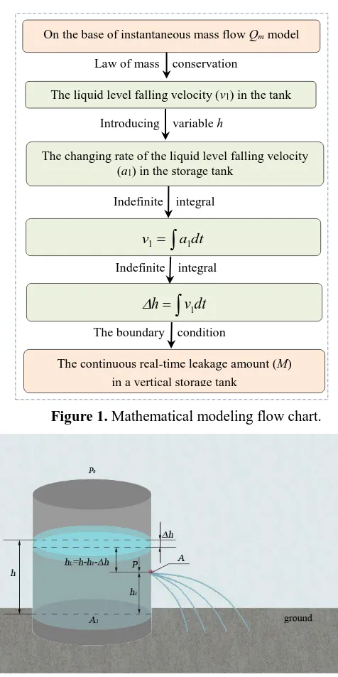
the flow speed of the liquid at the leaking hole. Basing on these two factors, the mathematical modeling 90
process for real–time leakage is shown in Figure 1. The schematic diagram of tank leakage is shown in 91
Figure 2. 92
93
Figure 1. Mathematical modeling flow chart. 94
95
Figure 2. Schematic diagram of tank leakage. 96
Law of mass conservation
On the base of instantaneous mass flow Qm model
Introducing variable h
The liquid level falling velocity (v1) in the tank
Indefinite integral
adt v1 1The boundary condition
vdt
h 1
The continuous real-time leakage amount (M) in a vertical storage tank
Indefinite integral
2.2.1. Liquid Level Falling Velocity 97
The liquid level in the tank is continuously decreasing when leakage occurs. The falling liquid level 98
velocity (v1) in the tank could be characterized with the height of the liquid that is higher than the 99
leaking point (hL). 100
The liquid flow velocity v at the leak point is firstly investigated and characterized with hL. At the 101
leaking point by the principle of mass conservation : 102
m
v
Q
Q (2)
103
v
Q A v
(
3) 104Equation (2) and Equation (3) are combined with Equation (1), thus the liquid flow rate (v) at the 105
leak point would be: 106
0
0 L
P-P
v C 2 g h
(4) 107
According to the basic law of conservation of mass, the quality of the liquid dropping in the tank 108
should be the same as that of the leaking–out liquid through the leaking point: 109
1 1
A v A v
(5) 110
Then the liquid level falling velocity (v1) in the tank could be obtained by Equations (4) and (5): 111
0
1 0 L
1
P-P A
v C 2 g h
A (6) 112
2.2.2. Changing Rate of the Liquid Level Falling Velocity 113
The changing rate of the liquid level falling velocity is dependent on several factors, such as the 114
diameter and height of the storage tank, the height of the liquid level in the storage tank, and the 115
diameter of the leaking hole. 116
The change in the liquid level above the leaking point is taken into account for the leakage at any 117
weak part of the tank: 118 h -h -h
hL 1 (7)
119
Equation (6) is squared, and combined with (7), then the solution would be: 120 0 1 2 1 2 0 1 p-p
g h-g h
v
h
-g A
2 C g
A (8) 121
Assuming that the leakage time is t, and the liquid level drop height Δh in the tank is found 122
derivation for v1: 123 1 1 1 1 a v dv dt dt h d dv h
d (9)
The changing rate of the liquid level falling velocity in the storage tank is solved by the Equations (9) 126 and (10): 127 2 1 0 1 A
a - C g
A (11) 128
2.2.3. Continuous Real–time Release Model M 129
The liquid level falling velocity (v1) is obtained via indefinite integral of the leak time by the 130
changing rate of the liquid level falling velocity in the storage tank (a1): 131
2 2
0 0
1 1 1
1 1
A C A C
v a dt - g dt - g t C
A A
(12) 132The integral constant C1 is found by the boundary condition (t = 0, v1 is the maximum value, and Δh 133
is zero), so: 134
0 0
1 1
1
A C P P
C 2 g h h
A (13) 135
The liquid level falling velocity (v1) is obtained by Equations (12) and (13): 136
2
0 0 0
1 1
1 1
A C P-P A C
v 2 g h-h g t
A A
( ) (14) 137
The liquid level drop height (Δh), as in the integral to the leak time t, could be characterized with the 138
liquid level falling velocity (v1): 139
2 2
0 0 0
1 1 2
1 1
A C P-P g t A C
h v dt 2 g ( h h ) t C
A 2 A
(15)140
The integral constant C2 is found by the boundary condition, if t = 0 and Δh = 0, then C2 = 0, and: 141
2 2
0 0 0
1
1 1
A C P-P g t A C
h 2 g ( h h ) t
A 2 A
(Δh ≤ h – h1) (16) 142
In summary, the continuous real–time leakage amount M of the vertical tank body is obtained under 143
the condition of M = ρV = ρA1Δh: 144 2 2 2 0 0 0 1 1
P-P g C A
M A C 2 g ( h h ) t t
2 A
(Δh ≤ h – h1) (17)
145
2.3. Model Constraints and Verification 146
The model constraints of the continuous real–time leakage model M are as follows: 147
(1) Before the time that the tank leakage occurs, that is, the leakage time tleakage start = 0, the liquid 148
level falling height Δhstart = h – h1 = 0 and the continuous true leakage amount Mstart = 0; 149
(2) When the leakage is completed (all liquid above the leak orifice flows out), that is, when the 150
tleakage end reaches at a certain time, the liquid level descending height Δhstart = h – h1 and the continuous 151
true leakage amount Mend = Mmax. 152
According to the actual liquid leakage and the model analysis, if the model constraints are 154
established for the continuous real–time leakage amount calculation with the time t as the variable, the 155
model is effective. 156
3. Model Application 157
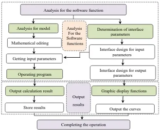
3.1. Model of Software Construction 158
C# language is used to develop the corresponding software in order to facilitate the model solving
159and application. After the software functions are analyzed, the model input parameters and their logical 160
relationships are determined, as well as the calculation output results and the graphic display functions, 161
and the software programming is completed. Figure 3 shows the software development flow chart. 162
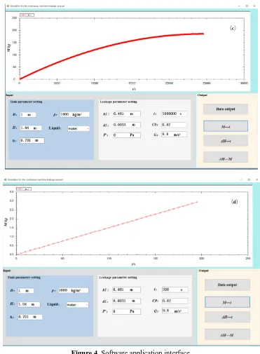
Figure 4 shows the software application interface, (a) and (c) of Figure 4 are the whole process 163
simulation amount, (b) and (d) of Figure 4 are the simulation amount of 200 s when the discharge 164
coefficient is 0.65 and 0.82 respectively under the experimental application. 165
166
Figure 3. Software development flow chart. 167
168
Analysis for the software function
Analysis for model
Mathematical editing
Determination of interface parameters
Getting input parameters
Operating program
Interface design for input parameters
Interface design for output parameters Analysis
For the Software functions
Output calculation result Graphic display functions
Store results Output the curves
Output
results
169
174
175
Figure 4. Software application interface. 176
3.2. Experimental Application 177
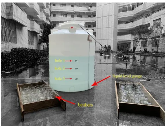
3.2.1. Leakage Tanks and Main Parameters 178
A tank was specifically designed and tested in order to evaluate the application of the model and the 179
operation of the software. The storage tank was made of PVC material and was a flat–bottom cylindrical 180
storage tank. The diameter of the bottom is D = 0.98 m, the total height is H = 1.45 m, and the height of 181
the cylindrical part is H1 = 1.04 m. The simulated leakage is through the small round holes. A plumb line 182
was taken with a steel ruler and a level meter, and the position of the leak holes was calibrated from 183
bottom up. The leakage hole diameter d was measured by averaging three measurements using vernier 184
leaking point to tank bottom h1, the initial liquid level height h, and the leakage hole shape are shown in 186
Table 1.The leaking test liquid is tap water. 187
Table 1. Data sheet of tank leakage Information. 188
hole number h/m h1/m shape of leakage hole d/m
1 0.701 0.617 circular 0.0033
2 0.701 0.4677 circular 0.0034
3 0.701 0.2677 circular 0.0034
The discharge coefficient C0 of 0.65 was generally applied for a circular leak hole, which was 189
introduced in the book about accident analysis [26]. C0 was not a clear value when tank body leaked in 190
AQ3046–2013. However it was clearly stated that the discharge coefficient was 0.62 for sharp orifices, 191
0.82 for rounded orifices, and 0.96 for straight orifices. So the theoretical values of C0 are 0.65 and 0.82 192
to be compared with experimental value [7]. 193
3.2.2. Experiment Requirement 194
Three repeated experiments were performed for each leak hole to better analyze the experimental 195
results. A pressure sensing liquid level gauge was added to the test to facilitate real–time measurement of 196
the leakage amount and real–time change of the liquid level. The relationship between the leakage time t 197
and the real–time discharge amount M within a certain leakage period according to the simulation results 198
of the model needs to be verified. 199
The leakage time step is 5 s during the experiments. The leaking liquid is collected and weighed in a 200
1000 mL beaker for 200 s. The leaking experiment site is shown in Figure 5. 201
202
Figure 5. Leaking experiment site. 203
4. Experimental Results and Discussion 204
4.1. Experimental Results 205
Each leakage orifice of No.1, No.2 and No.3 is tested for three times, and the discharge amount of 206
every time step is collected, weighted and recorded. Then every graph of three real–time leakage 207
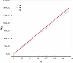
of hole 1, 2, and 3 on time respectively. Figure 6 shows that M1, M2 and M3 of hole 1 (d = 0.0033 m, h = 209
0.701 m and h1 = 0.617 m) are close to each other, especially for the first two experiments, and the graph 210
of M1 is the largest among three discharging experiments. The amount of M1 M2 and M3 is 1783.88 g, 211
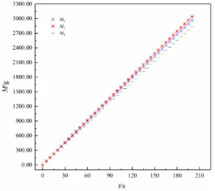
1760.22 g and 1657.20 g respectively when the leakage time is 200 s. Figure 7 shows that M1, M2 and M3 212
of hole 2 (d = 0.0034 m, h = 0.701 m and h1 = 0.4677 m) are nearly the same, especially for the first two 213
experiments, and the graph of M2 is the largest among three discharging experiments. The amount of M1 214
M2 and M3 is 2967.12 g, 3043.92 g and 2836.91 g respectively when the leakage time is 200 s. Figure. 8 215
shows that M1, M2 and M3 of hole 3 (d = 0.0034 m, h = 0.701 m and h1= 0.2677 m) have almost no 216
deviation, and the graph of M2 is the largest among three discharging experiments. The amount of M1 M2 217
and M3 is 4034.18 g, 4105.14 g and 4065.25 g respectively when the leakage time is 200 s. 218
219
Figure 6. Leakage amount curves of hole 1 with time (d = 0.0033 m, h = 0.701 m and h1 = 0.617m). 220
222
Figure 7. Leakage amount curves of hole 2 with time (d = 0.0034 m, h = 0.701 m and h1 = 0.4677m). 223
224
225
Figure 8. Leakage amount curves of hole 3 with time (d = 0.0033 m, h = 0.701 m and h1 = 0.2677m). 226
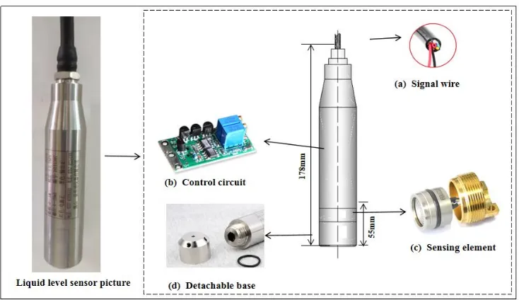
Figure 9 shows the structure of liquid level sensor. The actual liquid level differs by 5.5 cm since the 227
pressure sensing element is 5.5 cm from the bottom of the liquid level gauge. Figure 10 reveals the 228
relationship between the liquid falling level and the leakage time. The liquid level gauge shows that once 229
the leakage occurs, the leakage amount cannot be judged based on the change of the level gauge’s 230
232
Figure 9. Structure of liquid level sensor. 233
234
Figure 10. Relationship between liquid level drop and leakage time. 235
4.2. Discussion 236
4.2.1. Comparative Analysis of Leakage 237
The average amount Ma from three measurements of every discharging experiments is obtained to 238
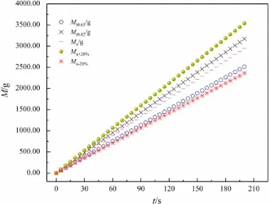
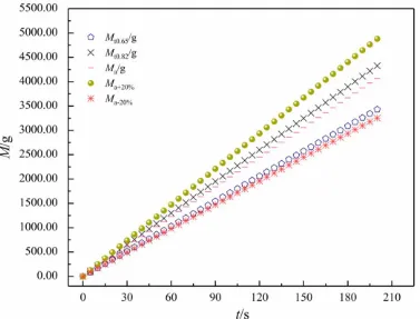
make a straightforward comparison. The positive deviation of the average by 20 % (Ma+20%), the negative 239
deviation of the average by 20 % (Ma–20%), and the theoretical leakage amount Mt0.65 (when C0 = 0.65) 240
and Mt0.82 (when C0 = 0.82) are illustrated in Figure 11, Figure 12 and Figure13. Ma and Mt are in the 241
intervals of Ma+20% and Ma–20% for hole 1, hole 2 and hole 3. Figure 11 shows that Ma, with the releasing 242
time of 200 s, is much larger than Mt0.65 but much closer to Mt0.82, and Mt0.65 is very close to Ma–20% when 243
the tank body is continuously released by hole 1 (d = 0.0033 m, h = 0.701 m and h1 = 0.617 m). Figure 244
12 reveals that Ma is much larger than Mt0.65, and close to Mt0.82. And the deviation between Mt0.65 and 245
Ma–20% is slightly separated when tank body is continuously released by hole 2 (d = 0.0034 m, h = 0.701 246
Furthermore the deviation between Mt0.65 and Ma–20% is almost the same when the tank body is 248
continuously released by hole 3 (d = 0.0033 m, h = 0.701 m and h1 = 0.2677 m). 249
250
Figure 11. Deviation leakage curves of hole 1 with time (d = 0.0033 m, h = 0.701 m and h1 = 0.617m). 251
252
254
Figure 13. Deviation leakage curves of hole 3 with time (d = 0.0033 m, h = 0.701 m and h1 = 0.2677 m). 255
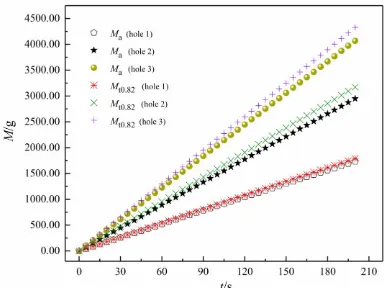
Discharge coefficient C0 is an important factor for calculation of theoretical leakage amount. C0, as a 256
theoretical discharge coefficient, is more suitable for the value of 0.82 under the condition studied in this 257
paper. Figure 14 gives the relationship between Ma and Mt for leaking hole 1, 2 and 3. It could be 258
straightly seen that the curves of Ma and Mt0.82 are almost completely coincident, which demonstrates that 259
theoretical value of 0.82 for discharge coefficient C0 is perfect for hole 1 (d = 0.0033 m, h = 0.701 m and 260
h1 = 0.617 m). The curves of Ma and Mt0.82 have a little overlap, which states that theoretical discharge 261
coefficient C0 should be corrected for hole 2 ( d = 0.0034 m, h = 0.701 m, h1 = 0.4677 m). The curves of 262
Ma and Mt0.82 have a slightly gap, which demonstrates that theoretical discharge coefficient C0 is 0.82 and 263
could be used for hole 3 (d = 0.0033 m, h = 0.701 m and h1 = 0.2677 m). 264
Consequently, the real–time leakage amount shows good linearity within 200 s leakage time. It can 265
be seen that Mt0.65 for leakage hole 1 is very close to the average deviation Ma–20% of the experimental 266
leakage amount, while the Mt for leakage hole No. 2 and No. 3 have a certain deviation from Ma–20%. All 267
the Ma of three holes are less than its Mt0.82 but closely to its Mt0.82, which demonstrates the validity of 268
270
Figure 14. Mt and Ma relationship of leakage hole 1, 2 and 3. 271
4.2.2. Effect of Liquid Level above the Leak Hole on Leakage Stability 272
The effect of the liquid level above the leak orifice on the leak hole is mainly reflected in the 273
pressure at the leak hole. Under the same meteorological conditions, the pressure at the leakage hole is P 274
– P0 + ρghL when the original liquid level h in the storage tank is unchanged and the distance between the 275
leakage hole and the ground h1 is different. The pressure at the leak hole is ρghL because the liquid 276
saturated vapor pressure (P – P0) is negligible for the regular pressure tank. The experimental leak 277
amount M of different leak holes varies with the instantaneous continuous flow velocity at the leak hole 278
changes because of the pressure. 279
The liquid level height hL above the leakage hole increases as the height h1 of the leakage hole 280
decreases, the liquid level change Δh in the storage tank will decrease slowly after the leakage occurs 281
when the original liquid level h is unchanged, so the change of pressure generated (ρghL) is small. 282
Therefore, the smaller the height h1 of the leakage hole is, the more stable the instantaneous continuous 283
flow velocity is and the larger leakage rate is. Obviously, during any time of the leakage, the real–time 284
leakage amount Ma of the No. 1 hole is the smallest, while the Ma for the No. 3 hole is the largest (Figure 285
14). This is verified by leak test data for holes NO. 1, 2 and 3. 286
4.2.3. Effect of Discharge Coefficient C0 on Leakage 287
The discharge coefficient C0 represents the dimensionless constant [27], which is obtained from the 288
complex function of the Reynolds number of the flow and the leak bore diameter [5, 28, 29, 30, 31]. The 289
Reynolds number is defined asRe
vd/
, where ρ is the liquid density, v is the liquid flow rate at the290
leak hole, d is the release hole diameter, and η is the dynamic viscosity coefficient of the liquid. Because 291
flow velocity of the leakage orifice changes continuously due to these factors. The original liquid level h 293
and the height h1 are different from each other, which leads to the corresponding Reynolds number Re 294
being different, so the discharge coefficient C0 is a non – constant value. In summary. C0 should be 295
adjusted according to the situation. In this paper, C0 is 0.82 for calculation of the theoretical leakage 296
amount Mt. 297
5. Conclusions 298
This paper focuses on the calculation of continuous real–time leakage amount after liquid hazardous 299
chemicals vertical tank releases. Through mathematical modeling, programming the model, and 300
experimental verification, the conclusions are obtained as follows: 301
(1) The mathematical model of continuous real–time release M and leakage time t is established by 302
the principle of mass conservation, which can improve the accuracy of continuous real–time release in 303
any leakage period after the tank body leaks. 304
(2) By experimental analysis of repeated leakage tests, the more stable the flow rate and the larger 305
the leak rate are under the condition that the higher the liquid level above the leakage hole (hL) is, the 306
greater the pressure on the leak hole is and the smaller the pressure changes at the leaking hole is. All the 307
Ma of three holes are less than its Mt0.82 but closely to its Mt0.82, the experimental results states that the 308
established model is effective. 309
(3) The discharge coefficient (C0) affects the accuracy of calculating leakage amount, which may 310
lead to deviations between Mt and Ma. The calculation accuracy of the continuous real–time leakage 311
amount M can be realized when the value of discharge coefficient is appropriate, and the reliability of 312
early warning prevention scheme can be provided for enterprise and government emergency rescue. 313
Author Contributions: J. H., L. Y. and Y.Z. conceived the initial and final design of the research work. 314
Q. Z., D. Z. and L.L. completed the experiments. A. L. simulated the model by C#. J. H. and D. Y. 315
analyzed the results and finished the manuscript's preparation. J. H., L. Y. and Y.Z. discussed the work 316
with the rest of the authors and refined the manuscript. J. H. wrote the paper with co-authors' support. 317
Funding: This study is supported by the key research and development program in Guangxi (category: 318
research and demonstration of key technologies for public safety and disaster prevention and mitigation, 319
Grant number: Guike AB16380288. 320
Acknowledgments: We would like to thank the anonymous reviewers for their time, work, and valuable 321
feedback. 322
Conflicts of Interest: The authors declare no conflict of interest.” 323
Nomenclature 324
M continuous real–time leakage amount g
Qm mass flow kg/s
Qv volume flow m3/s
ρ liquid density kg/m3
A1 bottom area of the tank m2
A area of leaking hole m2
P liquid pressure in the tank Pa
P0 environmental pressure Pa
g gravitational acceleration 9.8m/s2
h original liquid height in the tank before leakage m
h1 distance from the leaking point to tank bottom m
hL liquid height above the leaking hole m
Δh height at which the liquid level drops after the tank leaks m
v flow rate of the liquid at the leak hole m/s
v1 falling liquid level velocity in the tank m/s
a1 changing rate of the liquid level falling velocity in the storage tank m/s2
t leakage time s
C1 internal constant –
C2 internal constant –
V total volume of liquid leaked m3
D tank bottom diameter 0.98m
H total tank height 1.45m
H1 cylindrical part height 1.04m
d leakage hole diameter mm
M1 continuous leakage amount of the first experiment of every hole g
M2 continuous leakage amount of the second experiment of every hole g
M3 continuous leakage amount of the third experiment of every hole g
Ma average amount of the three experimental leakage of every hole g
Mt theoretical leakage calculation of every hole g
Mt0.65 theoretical leakage calculation (C0 = 0.65) of every hole g
Mt0.82 theoretical leakage calculation (C0 = 0.82) of every hole g
Ma+20% average value of the experimental leakage is positive by 20 % g
Ma–20% average value of the experimental leakage is negative by 20 % g
Re Reynolds number –
η dynamic viscosity coefficient of the liquid –
325
References 326
1. Cirimello, P. G., Otegui, J. L., Ramajo. D., et al. A major leak in a crude oil tank: Predictable and 327
unexpected root causes. Eng. Fail. Anal. 2019, 100, 456–469. 328
https://doi.org/10.1016/j.engfailanal.2019.02.005. 329
2. Hu, K., Zhao. Y. Numerical simulation of internal gaseous explosion loading in large–scale 330
cylindrical tanks with fixed roof. J. Thin–Walled Struct. 2016, 105,16–28. 331
http://dx.doi.org/10.1016/j.tws.2016.03.026. 332
3. S. M. Tauseef, Tasneem Abbasi, V. Pompapathi, S.A. Abbasi. Case studies of 28 major accidents of 333
fires/explosions in storage tank farms in the backdrop of available codes/standards/models for 334
safely configuring such tank farms. Process Saf. Environ. Prot. 2018, 120, 331–338. 335
4. Li Yunhao, Jiang Juncheng, Zhang Qingwu, Yu Yuan, Wang Zhirong, Liu Haisen, Shu Chi–Min. 337
Static and dynamic flame model effects on thermal buckling: Fixed–roof tanks adjacent to an 338
ethanol pool–fire. Process Saf. Environ. Prot. 2019, 127, 23–35. 339
https://doi.org/10.1016/j.psep.2019.05.001. 340
5. CPD. Purple Book: Guideline for Quantitative Risk Assessment. Committee for the Prevention of 341
Disasters, Hague, Netherlands, 2005a. 342
6. CPD. Red Book: Methods for Determining and Processing Probabilities. Committee for the 343
Prevention of Disasters, Hague, Netherlands, 2005b. 344
7. CPD. Yellow Book: Methods for the Calculation of Physical Effects. Committee for the Prevention 345
of Disasters, Hague, Netherlands, 2005c. 346
8. Liu, Q., Chen, Z., Liu, H., et al.. CFD simulation of fire dike overtopping from catastrophic ruptured 347
tank at oil depot. J. Loss Prev. Process Ind. 2017, 49, 427–436. 348
http://dx.doi.org/10.1016/j.jlp.2017.06.005. 349
9. Luo Tongyuan, Wu Chao, Duan Lixiang. Fishbone diagram and risk matrix analysis method and its 350
application in safety assessment of natural gas spherical tank. J. Clean. Prod. 2018, 174, 296–304. 351
https://doi.org/10.1016/j.jclepro.2017.10.334. 352
10. Lu, J., Yang, Z., Wu, H., et al. Model experiment on the dynamic process of oil leakage from the 353
double hull tanker. J. Loss Prev. Process Ind. 2016, 43, 174–180. 354
http://dx.doi.org/10.1016/j.jlp.2016.05.013. 355
11. Si, H., Ji, H., Zeng, X. Quantitative risk assessment model of hazardous chemicals leakage and 356
application. J. Saf. Sci., 2012, 50(7):1452–1461. https://doi.org/10.1016/j.ssci.2012.01.011. 357
12. He, B., Jiang, X. S., Yang, G. R., et al. A numerical simulation study on the formation and 358
dispersion of flammable vapor cloud in underground confined space. Process Saf. Environ. Prot., 359
2017, 107, 1–11. http://dx.doi.org/10.1016/j.psep.2016.12.010. 360
13. He, G., Liang, Y., Li, Y., et al. A method for simulating the entire leaking process and calculating 361
the liquid leakage volume of a damaged pressurized pipeline. J. Hazard. Mater. 2017, 332, 19–32. 362
http://dx.doi.org/10.1016/j.jhazmat.2017.02.039. 363
14. He, J.X., Yang, L.L., Liu, B., et al. 07.04. A calculation model based on continuous real–time 364
leakage of normal pressure vertical storage tank body. Application number of Chinese patent CN 365
201810724745.0. 2018. http://www.soopat.com/Patent/201810724745. 366
15. Zhen, X., Vinnem, J, E., Peng, C., et al., 2018. Quantitative risk modelling of maintenance work on 367
major offshore process equipment. J. Loss Prev. Process Ind. 2018, 56, 430–443. 368
https://doi.org/10.1016/j.jlp.2018.10.004. 369
16. DNV. UDM Verification Manual. DNV Software, UK, 2006. 370
17. DNV. PHAST Software Introduction [Online], Available: 371
https://www.dnvgl.com/services/hazard–analysis–phast–1675, 2016. 372
18. Dennis P. Nolan. Handbook of Fire and Explosion Protection Engineering Principles (Third 373
Edition). Dennis P. Nolan, 2014, 247–252. 374
19. Santiago Zuluaga Mayorga, Mauricio Sánchez–Silva, Oscar J. Ramírez Olivar, Felipe Muñoz 375
Giraldo. Development of parametric fragility curves for storage tanks: A Natech approach. Reliab. 376
Eng. Syst. Saf. 2019, 189,1–10. https://doi.org/10.1016/j.ress.2019.04.008. 377
20. China Coal Industry Publishing House, 2013. Guidelines for Quantitative Risk Assessment of 378
Chemical Enterprises (AQ/T 3046 – 2013), Beijing, 2013. 379
21. Kasai, N., Maeda, T., Tamura, K., et al.. Application of risk curve for statistical analysis of 380
backside corrosion in the bottom floors of oil storage tanks. Int. J. Pres Ves Pip, 2016, 141:19–25. 381
22. Shokrzadeh, A, R., Sohrabi, M, R. Buckling of ground based steel tanks subjected to wind and 383
vacuum pressures considering uniform internal and external corrosion. J. Thin Wall Struct. 2016, 384
108, 333–350. http://dx.doi.org/10.1016/j.tws.2016.09.007. 385
23. Amir R. Shokrzadehn, Mohammad R. Sohrabi.. Buckling of ground based steel tanks subjected to 386
wind and vacuum pressures considering uniform internal and external corrosion. Thin–walled 387
Struct., 2016, 108, 333–350. http://dx.doi.org/10.1016/j.tws.2016.09.007. 388
24. Manshadi S H D, Maheri M R. The effects of long–term corrosion on the dynamic characteristics 389
of ground based cylindrical liquid storage tanks. Thin–Walled Struct. 2010, 48(12): 888–896. 390
http://dx.doi.org/10.1016/j.tws.2010.05.003. 391
25. Mariusz Maslaka1, Michal Pazdanowskia, Janusz Siudutb, Krzysztof Tarsac. Corrosion durability 392
estimation for steel shell of a tank used to store liquid fuels. Procedia Engi. 2017, 172, 723–730. 393
http://dx.doi.org/10.1016/j.proeng.2017.02.092. 394
26. Jiang, J.C. Accident Investigation and Analysis Technology, second ed. Chemical Industry Press, 395
Beijing, 2011. 396
27. Crowl D A. Liquid discharge from process and storage vessels. J. Loss Prev. Process Ind. 1992, 397
5(2):73–80. https://doi.org/10.1016/0950–4230(92)80003. 398
28. DNV. DISC Theory Document. Palace House, 3 Cathedral Street, London SE19DE, UK, 2015. 399
http://www.dnv.com/software. 400
29. Masahiro Ishibashi. Discharge coefficient equation for critical–flow toroidal–throat venturi nozzles 401
covering the boundary–layer transition regime. Flow Meas. and Instrum., 2015, 44:107–121. 402
http://dx.doi.org/10.1016/j.flowmeasinst.2014.11.009. 403
30. Reader–Harris M. J., Sattary J. A.. The orifice plate discharge coefficient equation. Flow Meas. and 404
Instrum., 1990, 1(2):67–76. https://doi.org/10.1016/0955–5986(90)90031–2. 405
31. S. Essien, A. Archibong–Eso, L. Lao. Discharge coefficient of high viscosity liquids through 406
nozzles. Exp. Therm Fluid Sci., 2019, 103 :1–8.
407
https://doi.org/10.1016/j.expthermflusci.2019.01.004. 408