Representation, Recognition and Collaboration with Digital Ink
Representation, Recognition and Collaboration with Digital Ink
Rui Hu
The University of Western Ontario Supervisor
Dr. Stephen M. Watt
The University of Western Ontario
Graduate Program in Computer Science
A thesis submitted in partial fulfillment of the requirements for the degree in Doctor of Philosophy
© Rui Hu 2013
Follow this and additional works at: https://ir.lib.uwo.ca/etd
Part of the Graphics and Human Computer Interfaces Commons, Numerical Analysis and Scientific Computing Commons, and the Other Computer Sciences Commons
Recommended Citation Recommended Citation
Hu, Rui, "Representation, Recognition and Collaboration with Digital Ink" (2013). Electronic Thesis and Dissertation Repository. 1771.
https://ir.lib.uwo.ca/etd/1771
This Dissertation/Thesis is brought to you for free and open access by Scholarship@Western. It has been accepted for inclusion in Electronic Thesis and Dissertation Repository by an authorized administrator of
Graduate Program in
Computer Science
A thesis submitted in partial fulfillment of the requirements for the degree of
Doctor of Philosophy
The School of Graduate and Postdoctoral Studies The University of Western Ontario
London, Ontario, Canada
c
digital ink either in proprietary formats, which are restricted to single platforms and consequently lack portability, or simply as images, which lose important information. Moreover, in certain domains such as mathematics, current systems are now achiev-ing good recognition rates on individual symbols, in general recognition of complete expressions remains a problem due to the absence of an effective method that can reliably identify the spatial relationships among symbols. Last, but not least, existing digital ink collaboration tools are platform-dependent and typically allow only one input method to be used at a time. Together with the absence of recognition, this has placed significant limitations on what can be done.
In this thesis, we investigate these issues and make contributions to each. We first present an algorithm that can accurately approximate a digital ink curve by selecting a certain subset of points from the original trace. This allows a compact representation of digital ink for efficient processing and storage. We then describe an algorithm that can automatically identify certain important features in handwritten symbols. Identifying the features can help us solve a number of problems such as improving two-dimensional mathematical recognition. Last, we present a framework for multi-user online collaboration in a pen-based and graphical environment. This framework is portable across multiple platforms and allows multimodal interactions in collaborative sessions. To demonstrate our ideas, we present InkChat, a whiteboard application, which can be used to conduct collaborative sessions on a shared canvas. It allows participants to use voice and digital ink independently and simultaneously, which has been found useful in remote collaboration.
Keywords: Digital ink, InkML, handwriting recognition, mathematical handwrit-ing recognition, multimodal collaboration
Algebra for their generous help and valuable advice. It was an enjoyable experi-ence working with them. I am also grateful to the professors, Dr. John Barron, Dr. Mahmoud El-Sakka, Dr. Marc Moreno Maza, Dr. Roberbo Solis-Oba, and Dr. Olga Veksler, who have taught me throughout the years. Your lessons will be well-cherished.
Last, I wish to thank my family for their constant love and encouragement. For my parents who raised me with love and supported me in all my pursuits. For my wife who provided me considerate care during the final stage of the Ph.D. Thank you!
Table of Contents iv
List of Figures viii
List of Listings x
1 Introduction 1
1.1 Overview . . . 1
1.2 Representation of Digital Ink . . . 3
1.3 Recognition of Digital Ink . . . 7
1.4 Collaboration with Digital Ink . . . 9
I
Representation
11
2 Compact Representation of Digital Ink 12 2.1 Introduction . . . 122.2 Previous Work . . . 13
2.3 Objectives . . . 14
2.4 The Approximation Algorithms . . . 15
2.4.1 Problem Definition . . . 15
2.4.2 Algorithm . . . 18
2.4.3 Error Types . . . 18
2.4.4 Correctness . . . 20
2.4.5 Complexity . . . 20
4.1 Introduction . . . 35
4.2 SketchML to InkML . . . 38
4.2.1 SketchML to Archival InkML . . . 39
4.2.2 SketchML to Streaming InkML . . . 41
4.3 InkML to SketchML . . . 42
4.4 Implementation and Experiments . . . 43
4.5 Summary . . . 43
II
Recognition
44
5 Determining Points on Handwritten Mathematical Symbols 45 5.1 Introduction . . . 455.2 Determining Points . . . 46
5.3 Challenges . . . 46
5.4 Previous Work . . . 47
5.5 Objectives . . . 48
5.6 Handwriting Metrics . . . 49
5.7 Algorithms . . . 52
5.8 Experiments and Testing . . . 55
5.9 Use Cases . . . 59
5.10 Summary . . . 61
6.4 Experiments . . . 71
6.5 Summary . . . 76
III
Collaboration
77
7 Digital Ink Portability 78 7.1 Introduction . . . 787.2 Previous Work . . . 79
7.3 Objectives . . . 80
7.4 Portability of Software . . . 81
7.5 Portability of Digital Ink Data . . . 82
7.6 Summary . . . 83
8 Multimodal Collaboration 85 8.1 Introduction . . . 85
8.2 Previous Work . . . 86
8.3 Multimodal Collaboration . . . 88
8.3.1 Voice Input . . . 88
8.3.2 Handwriting Input . . . 89
8.3.3 Voice and Handwriting Multimodal Input . . . 89
8.4 Summary . . . 90
9 A Streaming Digital Ink Framework for Multi-Party Collaboration 91 9.1 Introduction . . . 92
9.2 Objectives . . . 92
9.3 Architecture . . . 93
9.3.1 The Collaboration Extension . . . 94
9.3.2 The Training Extension . . . 95
9.3.3 The Mathematical Recognition Extension . . . 96
10 InkChat: A Collaboration Tool for Mathematics 105
10.1 InkChat . . . 105
10.2 InkChat Support for Multimodality . . . 106
10.3 InkChat Support for Collaboration . . . 107
10.3.1 Communication . . . 107
10.3.2 Page Navigation . . . 107
10.3.3 Ink Editing . . . 107
10.3.4 Drag and Drop . . . 108
10.3.5 Real-Time Mirroring . . . 108
10.3.6 Session Recording and Playback . . . 110
10.4 Summary . . . 111
11 Conclusion 112
Curriculum Vitae 124
2.1 Approximation Error types. . . 19
2.2 Approximation of symbol “6” by specified number of pointsk. . . 21
2.3 Approximation of symbol “n” by cumulative error threshold ǫ. . . 22
2.4 The average time cost of using different error types in Algorithm 1. . 23
2.5 The average cumulative error of using different error types in Algorithm 1. 24 2.6 The average similarity between the approximated and original curve. 25 3.1 An example of Chinese calligraphy. . . 27
3.2 A simple stroke of Chinese calligraphy. . . 28
3.3 The model of Round Brush . . . 30
3.4 Filling the gap between two successive Round Brush ink points. . . . 31
3.5 The model of Tear Drop Brush . . . 31
3.6 Tear Drop Brush. (a) The tail end remains. (b) The tail end moves. . 32
3.7 An example of Chinese calligraphy using Tear Drop Brush. . . 33
3.8 The plot of Tear Drop Brush parameters . . . 34
4.1 SketchML elements. . . 37
4.2 Example of InkML Streaming style . . . 41
5.1 An example to illustrate the concepts of metric lines. . . 48
5.2 Baseline with (a) one determining point (b) multiple determining points. 49 5.3 X line and X height with (a) one, and (b) multiple determining points. 50 5.4 Ascender line and height . . . 51
5.5 Cap line and height . . . 51
5.6 Descender line and height . . . 52
5.7 Slant (θ) and width . . . 52
6.1 Baselines: (a) dq (b) dq (c) d (d) dq (e) dq (f) d . . . 65
6.2 Distance to average symbolvs the number of homotopy steps required. ∆s = 0.02, ∆y= 1%. . . 70
6.3 Distance to average symbolvs the number of homotopy steps required. ∆s = 0.02, ∆y= 3%. . . 71
6.4 Distance to average symbolvs the number of homotopy steps required. ∆s = 0.02, ∆y= 7%. . . 72
6.5 Distance to nearest neighbour vs the number of homotopy steps re-quired. ∆s = 0.02, ∆y= 1%. . . 74
6.6 Distance to nearest neighbour vs the number of homotopy steps re-quired. ∆s = 0.02, ∆y= 3%. . . 75
7.1 A cross-platform framework for digital ink applications . . . 82
9.1 InkChat architecture . . . 93
9.2 Collaboration framework . . . 94
9.3 Sessions with the stroke initiated by (a) the host and (b) the client. . 95
9.4 A client-server configuration with a stroke initiated by a client. . . 96
9.5 An example of diagramming in InkChat with Skype service. . . 100
9.6 The recognition interface . . . 101
9.7 An example of online learning and tutoring . . . 102
9.8 Examples of math and diagram collaboration. . . 103
10.1 InkChat page model . . . 108
10.2 An example of using Lasso in InkChat. (a) Selection (b) Drag (c) Drop 109 10.3 InkChat animation. . . 110
4.3 Example of conversion from SketchML to InkML streaming style. . . 42
1.1
Overview
Digital ink technology has experienced a tremendous growth over the past years. It has now been widely used by a variety of devices including Tablet PCs, PDAs, touch sensitive whiteboard systems, cameras and even smart phones. These devices accept digital ink input and pass it on to recognition software applications for interpretation. Systems can organize digital ink into documents or messages that can be stored for later reference or exchanged with other collaboration participants. These processes involve representation, recognition, and collaboration with digital ink. In this thesis, we investigate these aspects of digital ink and make contributions to each of them. Accordingly, this thesis is divided into three parts pertaining to aspects of digital ink representation, recognition and collaboration, each of which plays a critical role in digital ink technology.
conse-One of the sub-problems in handwriting recognition is to interpret handwritten math-ematics. This is a very challenging problem in that mathematical input is two-dimensional, with elements of both writing and drawing. Moreover, writing mathe-matical symbols typically does not follow simple baselines and the symbols may be written in different sizes, such as subscripts and superscripts. This makes it difficult to reliably identify the spatial relationships among symbols. To solve this problem, it requires an effective method that can accurately differentiate between fluctuations in positioning and intentional sub- or super-scripts, which in return will benefit hand-writing recognition. This will be discussed in Section 1.3.
Pen input is conducive to writing in mathematics since most mathematical no-tations are two dimensional. According to a study [1], pen input of mathematics is about three times faster and two times less error-prone than standard keyboard and mouse input. We can improve the efficiency even further by incorporating it into a multi-party, collaborative environment where multiple participants, who may be geo-graphically separated, could write or draw, for instance, on a shared canvas. This has great potential to enhance distance collaboration between mathematicians, allowing them to share a common virtual space and interact with it in the most natural ways, just like having a discussion in the same room. With the widespread availability of pen-enabled devices, developing such a collaborative environment has garnered much interest from researchers in academia. This will be discussed in Section 1.4.
Within the broad areas of representation, recognition and collaboration, this thesis investigates a number of specific sub-problems. We identify these briefly and then continue with a general discussion of the context in which they arise.
• Chapter 2 describes an algorithm to obtain compact representation of digital ink.
• Chapter 3 investigates the suitability of InkML to flexibly represent sophisti-cated digital ink and proposes two brush models to demonstrate our ideas.
• Chapter 8 examines the design issues in incorporating multimodal interactions in mathematical collaboration.
• Chapter 9 proposes a streaming digital framework that is suitable for multi-party collaboration.
• Chapter 10 presents InkChat, a whiteboard application, to demonstrate our ideas.
It is expected that, by solving these sub-problems, it will greatly benefit digital ink applications. In the remainder of the chapter, we will further introduce each of the sub-problems, respectively.
1.2
Representation of Digital Ink
Data Representation
Existing handwriting recognition methods are typically based on representing char-acters by sequences of points, each of which contains xand y values in a rectangular coordinate system. This representation is readily available from a digital pen which samples points from a traced curve with a certain frequency and outputs the sequence of their coordinates in real time.
programming. The main advantage of the algorithm is that it is independent of the choice of compatible error function and has a cost linear in the number of points. This algorithm can be used to compact the representation of digital ink data while preserving the shape of curves.
A flexible format that can accurately represent digital ink is essential for pen-enabled software applications. Modern devices have reached maturity to support different drawing and writing activities, e.g. diagramming and digital painting, by providing additional information such as pen tilt angle, pen tip force, timestamp,etc. However, few digital ink formats allow recording the additional information. After considering various alternatives, we have arrived at a design of using InkML [3] to represent digital ink. InkML has the advantage of being a W3C standard format. It provides application-defined channels to support sophisticated digital ink representa-tion. To demonstrate our ideas, we present two virtual brush models, Round Brush and Tear Drop Brush. Both models can be used to improve the rendering quality of digital ink. The Tear Drop Brush has been adopted into the InkML standard at our suggestion.
conver-tion), which try to convert device resolution after the fact. These methods replace the captured data with made up data that might have been captured on a different device. To address this issue, we adopt an approach that can represent handwritten symbols in the space of coefficients of a functional approximation. This approach has been used in earlier work [7, 8, 9, 10].
We consider an ink trace as a segment of a plane curve (x(s),y(s)), parameterized by Euclidean arc length, s,
ds2 =dx2
+dy2
This parameterization has been found to lead to good recognition and makes intuitive sense, since it gives curves that look the same the same parameterization [7]. Given a digital ink trace (x(s), y(s)) and an approximating basis {Bi(s)}i=0,...,d, we represent the trace using the coefficients xi and yi from
x(s)≈ d
X
i=0
xiBi(s) y(s)≈ d
X
i=0
yiBi(s)
It is convenient to choose the functions Bi(s) to be orthogonal polynomials, e.g. Chebyshev, Legendre or some other polynomials. By choosing an appropriate family of basis polynomials to high enough degree, the approximating curve can be made arbitrarily close to the original trace.
We have found a Legendre-Sobolev basis allows approximating curves to have the desired shape for relatively low degrees. These may be computed by Gram-Schmidt orthogonalization of the monomials {si} with respect to the inner product
hf, gi=
Z b
a
f(s)g(s)ds+µ
Z b
a f′
(s)g′
(a) (b)
Figure 1.1: Approximation using Legendre-Sobolev series. (a) Original. (b) Approximated using series of degree 12 with µ= 1/8.
(a) (b)
Figure 1.2: Another example of approximation using Legendre-Sobolev series. (a) Original. (b) Approximated using series of degree 12 with µ= 1/8.
the analysis of the spatial relationships between symbols challenging as it introduces various ambiguities. For example, whether a particular symbol is lowercase “p” or an uppercase “P” makes the difference between a subscripted pq or the juxtaposed P q. To help solve the problem, it requires an effective algorithm that can accurately dif-ferentiate between fluctuations in positioning and intentional sub- or super-scripting over a baseline. In order to accomplish this, we need to understand the scale and relative positioning of individual symbols. Therefore, it becomes necessary to identify the location of certain expected features, such as the location of baseline, which are typically defined by particular points in the symbols. These particular points occur at different locations in different symbols, and their precise locations may vary in different handwriting samples of the same symbol. For example, the baseline of a lower “p” would be identified by the lowest part of the bowl, ignoring the descender. In contrast, the baseline of lowercase “k” would be identified by the toes. We refer to a point such as this, that determines the height of a metric line, as a determining point.
To address this problem, we present an algorithm that can automatically iden-tify the determining points in handwritten symbols. Knowing the determining points of each symbol can help us solve a number of problems. For example, one can use the determining points to improve two-dimensional mathematical recognition. By comparing the baseline locations and the sizes of adjacent symbols, one can identify subscripts and superscripts (e.g. S2, S2, S2) with more confidence. Another ap-plication is in handwriting neatening. Since handwritten symbols often come with variations in alignment and size, certain transformations based on determining points can be applied to obtain normalized samples while preserving the original writing style. In contrast to existing methods, which treat digital ink traces as a collection of discrete points, this algorithm relies on interpreting ink traces as single points in a functional space. This allows device independence, on one hand, and a simple for-mulation of homotopic deformation, on the other. To evaluate the performance of the algorithm, we test it against a database of handwritten mathematical characters. The experiments show promising results.
ware reduces the ability of the individual or the group to master its use. If any of the members has difficulty, efficiency of the whole team suffers. Second, existing sys-tems typically allow only one input method to be used at a time. For example, in Microsoft OneNote, one can either type or draw, but not simultaneously. This places strong limitations on what can be done. For example, it becomes quite awkward to explain an activity while it is being performed. Last, but not least, we believe that the synergy of pen-based collaboration and recognition of mathematical input can enhance the efficiency of online interaction. Nevertheless, there is no technology that allows to capitalize on both simultaneously: some software handles recognition without the ability for real-time sharing, e.g. the Maple computer algebra system [13], while others provide sharing, but no mathematical recognition, e.g. Microsoft OneNote [14], Calliflower [15] or Dabbleboard [16].
Part I
Chapter 2
Compact Representation of
Digital Ink
Digital ink curves are typically represented as series of points sampled at certain time intervals. We are interested in the problem of how to select a minimal subset of sample points to approximate a digital ink curve within a given error bound. We present an algorithm to find an approximation with a specified number of points and providing the minimum cumulative error. Alternatively, it may be used to select the minimum number of points required to satisfy an error bound. This chapter is based on the article “Optimization of Point Selection on Digital Ink Curves” [17] co-authored with Stephen M. Watt, that appeared in the proceedings of the 13th International Conference on Frontiers in Handwriting Recognition.
2.1
Introduction
straight line).
2.2
Previous Work
continuous curve may be approximated by a piecewise linear function with vertices on the curve. Decreasing the arc length discrepancy by adding points to a piecewise linear approximation decreases all the usual error measures and cannot increase them.
We present an algorithm to find an optimal point selection to approximate a piecewise linear curve. It can be used in two ways:
• Given a digital ink curve consisting of n ≥ 2 points and a specified number of points 2 ≤ k ≤ n, the algorithm selects a subset of k points such that the arc length discrepancy between the approximation and the original curve is minimized.
• Given a digital ink curve and a bound on arc length discrepancy, the algorithm selects a subset of points of minimum number required to approximate the curve to within that bound. That is, no smaller subset of the original points can achieve the bound.
Both uses are globally optimal and can be applied to both open and closed, planar and space curves.
The method can be applied when other error measures are of interest. In this case, though fast and good, the point selection is not guaranteed to be optimal. We have used this method with a variety of error types used in prior work, including the arc-chord length difference, maximal height, average height, which in turn measure the difference between the curve length and the chord length, the maximal height from the curve to the chord, and the average height from the curve to the chord. All of these errors are computed on each curve segment.
points k, 2 ≤ k ≤ n, how can we select the k points such that the cumulative error between the approximation and the original curve is minimized?
• Given a digital ink curve consisting of n ≥ 2 points and a cumulative error threshold ǫ ≥0, how can we select the minimum number of points required to approximate the curve such that the cumulative error is less than or equal toǫ?
Both problems can be seen as graph problems. Given a digital ink curve consisting ofn points, we first assign an index to each point. A weighted DAG (directed acyclic graph) G(V, E) can be constructed from these points, where
(
V = {vi | 0≤i≤n−1}
E = {(vi, vj) | 0≤i < j ≤n−1}
(2.1)
The set V contains n vertices, with vi corresponding to the i-th point pi on the digital ink curve. The DAG will be constructed to have a unique source (vertex with no inbound edge) and a unique sink (vertex with no outbound edge). The source corresponds to the initial point p0 and the sink corresponds to the final point pn−1. The weight of each edge is defined as:
w(vi, vj) = errorF n(pi, pj) (2.2)
S ← {};
// The minimum weight table D←(k+ 1)×n matrix; // Path
P ←(k+ 1)×n matrix; // Initialization
for j ←1 to n−1do
D2,j ←w(v0, vj); P2,j ←0;
// Compute the rest of D
for m←3 to k do
for j ←m−1 to n−1do
min weight← ∞;
for i←m−2 to j−1 do
weight←Dm−1,i+w(vi, vj); prior vertex index ←0;
if weight < min weight then
min weight←weight; prior vertex index← i; Dm,j ←min weight;
Pm,j ←prior vertex index;
// Restore the path vertex index←n−1;
for i←0to k−1 do
S ←S∪ {vertex index}; vertex index←Pk−i,vertex index
return S
P ←(n+ 1)×n matrix;
// The smallest m that makes Dm,n−1 ≤ǫ m∗ = 2;
// Initialization
for j ←1 to n−1do
D2,j ←w(v0, vj); P2,j ←0;
if D2,n−1 > ǫthen
// Compute the rest ofD
for m←3 to n do
for j ←m−1 to n−1do
min weight← ∞;
for i←m−2 to j−1 do
weight←Dm−1,i+w(vi, vj); prior vertex index← 0;
if weight < min weight then
min weight←weight; prior vertex index←i;
Dm,j ←min weight;
Pm,j ←prior vertex index;
if Dm,n−1 ≤ǫ then m∗ ← m;
break;
// Restore the path vertex index←n−1;
for i←0to m∗−1 do
S ←S∪ {vertex index};
vertex index←Pm∗−i,vertex index
we assign
D2,j =
(
∞ if j = 0
w(v0, vj) if 0< j ≤n−1
For m≥3, Dm,j can be computed as:
Dm,j =
min
m−2≤i<j{Dm−1,i+w(vi, vj)} if j ≥m−1
∞ otherwise
Therefore, finding the minimum cumulative error of a k-point approximation is simply to compute Dk,n−1, wherek is the specified number of points andn−1 is the index of the final point on the original curve. The complete algorithm to select thek points is shown in Algorithm 1.
Similar to Algorithm 1, finding an approximation consisting of the minimum number of points such that the cumulative error is within a given threshold, ǫ, is achieved by exiting the loop with a break statement. We keep computing Dm,n−1 for m = 2. . . n until we find the firstm that makes Dm,n−1 ≤ ǫ. For additive errors, the m is guaranteed to exist as the cumulative error decreases when more points are selected and reaches 0 when all points are selected. The complete algorithm is laid out in Algorithm 2.
2.4.3
Error Types
(c)
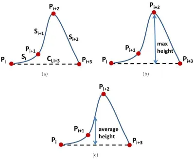
Figure 2.1: Error types: (a) Arc-Chord Length Error, (b) Maximal Height Error, and (c) Average Height Error. The curve is constructed using cubic spline interpolation.
the approximated curve, which reflects the global deviation from the original one. As digital ink curves may be generated in different scales, we normalize each by its arc length in order to evaluate the error fairly.
As we are interested in minimizing the global deviation error, we choose error types based on three criteria. A good type of error should be computationally efficient, additive, and has a natural meaning in geometry. In this thesis, we consider three types: Arc-Chord Length Error, Maximal Height Error, and Average Height Error.
2.4.4
Correctness
Selecting the m-th point is a process of computing Dm,n−1, where n−1 is the index of the final point on the original digital ink curve. Since
Dm,n−1 = min
m−2≤i<n−1{Dm−1,i+w(vi, vn−1)},
we can recursively computeDm,n−1,m= 3. . . nusing dynamic programming with the given initial conditionD2,i=w(v0, vi), 0< i≤n−1. This is a particular application of the Principle of Optimality [22] and Dm,n−1 will be the minimum cumulative error of the approximation consisting ofm points.
Since the Arc-Chord Length error is additive, the matrix D has the following properties: with the increase of m, Dm,n−1 decreases and reaches 0 when m = n. But for the other two types errors, the matrix D may not have the property that Dm,n−1 ≤ Dm′,n−1 when m′ ≥ m. However, since Dn,n−1 is 0 in either case, we can always use the algorithm to find the solution.
2.4.5
Complexity
The complexity to find the k-point approximation is O(kn2
). To see this, note we are computing a matrix. To selectk points, it is necessary to compute k rows. Since each row has n entries, we have a total cost of O(kn2
). Finding an approximation within a given cumulative error threshold ǫ, in the worst case that all points on the original digital curve need to be selected, giving complexity O(n3
).
(a) k= 5,e= 0.052 (b)k= 10,e= 0.013
(c) k= 15,e= 0.005 (d)k= 20,e= 0.002
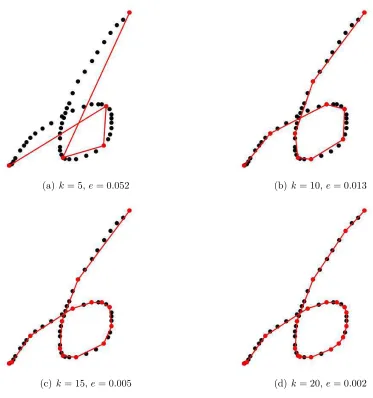
Figure 2.2: Approximation of symbol “6” by specified number of pointsk. The black points are the points on the original curve. The red points are the approximation. The error is the arc-chord length error. We use e to denote the cumulative error.
2.5
Experiments
Figure 2.2 shows an example of applying Algorithm 1 to a digital ink curve. The digital ink curve consists of 55 points which are marked as black dots. The red dots are the selected points in the approximation. The error adopted here is the Arc-Chord Length Error. Increasing the number of selected points from 5 to 20, the approximation approaches the original digital ink curve quickly.
(a) ǫ= 0.05,s= 6,e= 0.0459 (b) ǫ= 0.02,s= 9,e= 0.0182
(c) ǫ= 0.01,s= 12,e= 0.0093 (d) ǫ= 0.005,s= 16,e= 0.004
(e) ǫ= 0.002,s= 19,e= 0.0018 (f) ǫ= 0.001,s= 23,e= 0.0009
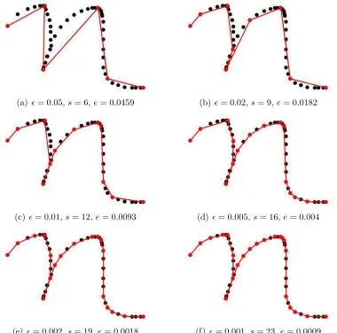
Figure 2.3: Approximation of symbol “n” by cumulative error thresholdǫ. The black points are the points on the original curve. The red points are the approximation. The error is the Arc-Chord Length Error. We use s and e to denote the number of selected points and the cumulative error, respectively.
points in the approximation. The error adopted here is the Arc-Chord Length Error. As we decrease the error thresholdǫ, more points are selected in order to restrict the cumulative error withinǫ. When the error threshold drops to 0.001, the approximation is almost as the same as the original digital ink curve. But the number of points selected in the approximation is only half of the size of the original.
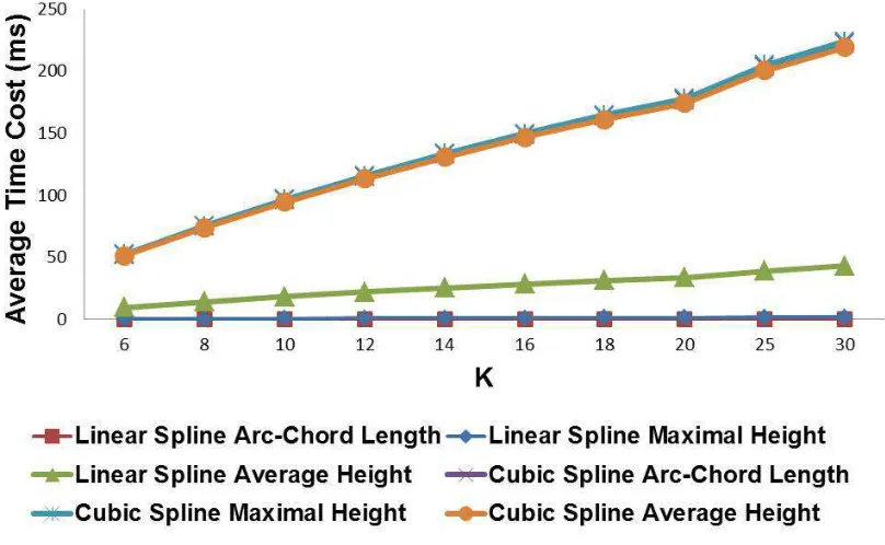
Figure 2.4: The average time cost of using different error types in Algorithm 1.
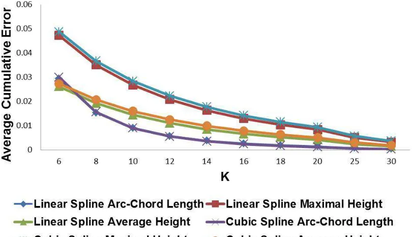
in these symbols. We constructed digital ink curves from these strokes using linear and cubic spline interpolation since they are commonly used in the area of digital ink rendering, handwriting recognition, and handwriting neatening. All of the curves were normalized by arc length in advance. We measured the average time cost in mil-liseconds and average cumulative error (relative to the trace length) on each digital ink curve. Figure 2.4 shows the average time cost of applying different error types in Algorithm 1. We see that the Arc-Chord Length Error outperforms the others in both linear and cubic spline cases. Figure 2.5 shows the average cumulative error of applying different error types in Algorithm 1. With the increase of the specified number of points, the average cumulative errors of all types drop dramatically, but takes longer to compute.
approxi-Figure 2.5: The average cumulative error of using different error types in Algorithm 1.
mated curve and original one. Since the two curves share the same initial and final points and our point selection is a subset of the entire point set, one can compute the difference between the arc length of the approximated curve and of the original curve. A smaller difference suggests a higher similarity and a better approximation. Figure 2.6 shows the average similarity which is defined as the arc length of the ap-proximated curve divided by the arc length of the original curve. With the increase of the specified number of points, the arc length of the approximated curves approaches the arc length of original curve quickly.
2.6
Summary
Figure 2.6: The average similarity between the approximated curve and original curve.
Error, the Maximal Height Error, and the Average Height Error. These were chosen for their computational efficiency and natural geometric meaning. Our experiments have shown that the Arc-Chord Length Error outperforms the others in terms of average time cost in both linear and cubic spline cases.
Chapter 3
Flexible Representation of
Sophisticated Digital Ink
Modern devices have reached maturity to support different drawing and writing activ-ities, e.g. diagramming and digital painting, by providing additional information such as pen tilt angle, pen tip force, timestamp,etc. However, few digital ink formats allow recording these additional information. In this chapter, we investigate the suitability of InkMl to represent sophisticated digital ink. InkML is a W3C standard format. It provides application-defined channels to support sophisticated digital ink representa-tion. To demonstrate our ideas, we present two virtual brush models, Round Brush and Tear Drop Brush. Both models can be used to improve the rendering quality of digital ink. The Tear Drop Brush has been adopted into InkML at our suggestion. This chapter is based on my master thesis [24].
Xizhi Wang, a well known calligrapher [25].
3.1
Introduction
Although digital ink technologies have evolved over years, the “brushes” used by dig-ital ink applications are still simpler than real brushes. These brushes are normally two dimensional, only recording X and Y coordinates. Even in sophisticated appli-cations, brush tip shapes tend to be at most ellipses or rectangles with a major and minor dimension and perhaps an angle. Few of them provide support to record ad-ditional information such as pen tilt angle, pen tip force, timestamp, etc., which are essential when simulating more complex writing instruments. With the widespread application of pen-based devices, it has become increasingly popular to render digital ink strokes with different styles. This is particularly useful when aesthetic and deco-rative effects are desired. Many Asian writing systems use a round brush with long bristles as the writing implement. While the elliptical or rectangular contact shapes may be sufficient to model writing with pens, they cannot represent the characteris-tics of a physical brush. Take Chinese calligraphy as an example, as shown in Figure 3.1, since the brush is made of soft bristles, there are abundant width variations. The width variations even exist in a single stroke. For instance, in Figure 3.2, the stroke is fat at the beginning as writers pressed hard when the brush tip dropped on the paper. Then it become thinner while the brush was moving. As soon as the brush reached the end of the stroke, the tip suddenly turned back and the stroke got fat again due to the delay of the long brush tail.
Figure 3.2: A simple stroke of Chinese calligraphy.
[26]. He described an investigation into a realistic model of painting and proposed a method which can be used to simulate the properties of wet paint brush. Wong and Ip [27] presented an method to simulate the physical process of brush stroke creation. This method uses a parameterized model which captures the brush’s 3D geometric parameters, the brush bristle properties as well as the variations of ink deposition along a stroke trajectory.
Our work is similar to those in that we all keep track of each ink point and calculate its contour to simulate brush properties. Our work is also apart of those as we are using InkML, a W3C standard, to represent and render digital ink.
In this chapter, we present two virtual brush models,Round Brush andTear Drop Brush, to render digital ink in different styles. The Round Brush may best be used for diagramming while the Tear Drop Brush may be suitable for digital painting or East Asian Calligraphy. Both brush models have been integrated into InkChat [28], a whiteboard application which allows conducting multi-party collaboration.
The remainder of this chapter is organized as follows. In Section 3.2, we explain how to represent sophisticated digital ink using InkML. Section 3.3 presents the brush models. In Section 3.4, we summarize the chapter with a brief discussion and suggest a few directions of future work.
3.2
InkML Representation
information such as location, pen tip pressure, timestamp and tilt angle. To render it with a particular brush property, we can simulate the dynamic brush shapes by calculating the contour at each ink point.
To demonstrate our ideas, we have developed two virtual brush models.
3.3
Brush Models
Calligraphy cannot be rendered using simple lines or curves due to the stroke width variations. We thus use a different approach: we calculate the dynamic brush shape at each point while the brush is moving. Obviously, different brushes result in different 2D contours. Even using the same brush, different pressure may cause contour size and shape variations. Therefore, after capturing the digital ink from pen-based device, we convert it to brush-specific parameters and then render it according to the brush type.
The first brush we developed is the Round Brush. We have also developed a more sophisticated one, Tear Drop Brush, which can be used to simulate Chinese calligra-phy. The following two sub-sections illustrate the two brush models, respectively.
3.3.1
Round Brush
(x , y )
Figure 3.3: The model of Round Brush
which is a function of pen tip pressure. In general, the harder you press the brush, the larger the circle. In our model, the radius of the circle r is linearly proportional to the pressure p, i.e.
r =kp,
where k is a heuristic constant.
Pen-based devices work under certain sampling rates. A higher sampling rate indicates it can sample more ink points in a unit time and therefore leads to a greater chance that two successive circles would overlap. A lower sampling rate indicates it can sample fewer ink points in a unit time and leads to a smaller chance that two successive circles would overlap. In addition, if the brush moves fast, the chance of overlapping would correspondingly decrease. Practically two successive circles do not overlap if the brush is moving. Even if they are overlapped, there is a great chance that they are not fully overlapped. As long as full overlap does not exit, there will be a gap between each pair of successive circles. In order to obtain a smooth rendering, we fill the gaps by calculating the external tangents and coloring the area determined by the four tangent points, as shown in Figure 3.4.
3.3.2
Tear Drop Brush
(x, y)
l
r
θ
Figure 3.5: The model of Tear Drop Brush
out and the ink mark would become a fat round dot again. Based on this idea, we use five parameters to model the Tear Drop Brush, as shown in Figure 3.5. x and y indicate the position of the ink point, r represents the head radius, θ indicates the rotation angle of the tail, and l measures the tail length, the distance from the circle centre to the tail end.
In principle, the head radius should be a function of pressure. The harder you press the brush, the larger the radius would be. In our approach, we set the radius r to be directly proportional to the pressure p, i.e.
r =kp,
where k is a heuristic constant.
0000000
1111111
2 2
(x , y )
1 1
(x , y )
(a) 0000000000 0000000000 0000000000 0000000000 0000000000 0000000000 0000000000 0000000000 0000000000 0000000000 0000000000 0000000000 0000000000 0000000000 0000000000 0000000000 0000000000 1111111111 1111111111 1111111111 1111111111 1111111111 1111111111 1111111111 1111111111 1111111111 1111111111 1111111111 1111111111 1111111111 1111111111 1111111111 1111111111 1111111111 l1 r1 2 2
(x , y )
r2
1 1
(x , y )
L
L
(b)
Figure 3.6: Tear Drop Brush. (a) The tail end remains. (b) The tail end moves.
value depends on the distance between old tail end and the position of the new ink point.
Figure 3.7: An example of Chinese calligraphy using Tear Drop Brush.
In the implementation, we retrieve coordinates and pen tip pressure at each ink point from a Wacom tablet running on Ubuntu 8.10. We convert it to the Tear Drop Brush parameters and then save them into InkML points (x, y, r, θ,l). An example image of the Tear Drop Brush calligraphy can be seen in Figure 3.7. Figure 3.8 shows the plot of the first stroke of Figure 3.7.
3.4
Summary
Our work is an attempt to render digital ink with calligraphic properties. We have found a simple mathematical model to be sufficient to represent writing with a round, bristled brush. Our model is able to portray a good approximation to the contact shape of a brush being dragged along the writing surface, depositing ink with changes in pressure and direction. This “tear drop” contact shape has been adopted into InkML at our suggestion.
(a) The ink stroke to plot (in red). X C o o r d in a te 150 200 250 300 350 400 450 500 550 Absolute Time
1.124e+07 1.124e+07 1.124e+07 1.124e+07 1.124e+07 1.124e+07
(b) The plot of xcoordinates
Y C o o r d in a te 100 200 300 400 500 600 700 Absolute Time
1.124e+07 1.124e+07 1.124e+07 1.124e+07 1.124e+07 1.124e+07
(c) The plot ofy coordinates
H e a d R a d iu s 0 2 4 6 8 10 12 Absolute Time
1.124e+07 1.124e+07 1.124e+07 1.124e+07 1.124e+07 1.124e+07
(d) The plot of the head radius
T a il L e n g th 5 6 7 8 9 10 11 12 13 14 Absolute Time
1.124e+07 1.124e+07 1.124e+07 1.124e+07 1.124e+07 1.124e+07
(e) The plot of the tail length
Digital Ink
The MIT Sketch Markup Language (SketchML) and the Ink Markup Language (InkML) are both used for sketch data representation. Techniques for exchanging sketch data between the two formats, however, are currently not readily available. In this article, we present a data binding solution for two-way conversion between SketchML and InkML. We show how to transform SketchML files to InkML archiv-ing and streamarchiv-ing style. This allows sketch data to be used in collaborative en-vironments where real-time sharing is desired. In the reverse conversion, we bind InkML elements to SketchML elements. This makes sketch data that is represented by InkML available to existing SketchML applications. We have tested these ideas in a shared whiteboard application and found them to perform well. This chapter is based on the article “From MIT SketchML to InkML, or There and Back Again” [31] co-authored with Stephen M. Watt, that presented at 10th IAPR International Workshop on Document Analysis Systems.
4.1
Introduction
formats, similar in that they both record trace information, but otherwise quite dif-ferent. This chapter examines the question of what is involved in converting between these formats. Before describing the technical challenges and our solutions, we first set the stage with some basic ideas.
InkML (Ink Markup Language) is an open and up-to-date recommendation stan-dard which is proposed by the W3C (World Wide Web Consortium). It can be used by digital ink applications for multiple purposes. n particular, it supports digital ink sharing based on the concept of context [32]. The context is represented by the <context> element which contains various aspects of real-time scenario, including <canvas>, <canvasTransform>, <traceFormat>, <inkSource>, <brush> and <timestamp>, which in turn specifies the canvas, canvas transformation, trace for-mat, ink source properties, brush properties and time stamp.
SketchML (Sketch Markup Language) is an XML-based open format which was developed by the Design Rationale Group at MIT. It provides a collection of elements to represent user’s sketch as well as other meta information such as the study and the domain that the sketch was created for. It enables stroke grouping and annotation by allowing for the creation of the <shape> element. SketchML is useful in sketch data representation and annotation [33]. However, it lacks support for sketch sharing which is critical in many collaborative scenarios. These scenarios, such as classroom teach-ing, distance education, work-group meetteach-ing, and collaborative document annotation, typically involve multiple participants, which is complicated compared with the sin-gle user case. The application in these scenarios could be even more restricted when the collaborative environment is heterogeneous. The restrictions stem not only from differences between operating systems and platforms but also from the differences in characteristics of the pen devices, such as channel properties, screen resolution and so on.
conversion is not straightforward. The organizations of the elements within the two formats are different. Hence, they impose different requirements for markup proces-sors and generators and give different computational complexities for certain oper-ations. In SketchML, contextual information are delivered by the attributes of the <shape> element which represents a series of strokes. All the ink points associated with the strokes are given by references to the <point> elements which are typi-cally stored separately from the <shape> element. This is opposite to the InkML format. In InkML, contextual information are retrieved from strokes and stored apart. Depending on scenarios, the contextual elements may appear either within <definitions>element or prior to<trace>/<traceGroup> elements. References to the contextual elements are made by the <contextRef> and the <brushRef> attributes of the <trace>/<traceGroup> element. The<trace>/<traceGroup> element carries explicit coordinate values instead of references to ink points. There-fore, this conversion problem is to transform the SketchML format to the InkML format and vice versa in efficient ways. In an abstract view, this transformation can be seen as semantically binding elements between the two formats.
In this chapter, we present a technique to interchange sketch data between the SketchML format and the InkML format. By converting from SketchML to InkML, we make SketchML data acceptable by digital ink applications that support InkML. We also exploit the InkML streaming features so that sketch can be shared in real time between participants, who may be in the same room or across the planet. By converting from InkML to SketchML, we make sketch data that is represented by InkML compatible to existing SketchML applications.
technique to convert sketch data from the SketchML format to the InkML format. In section 4.3, we discuss the technique of the reverse conversion, from the InkML format to the SketchML format. In section 4.4, we present a sketching interface implementation to demonstrate our ideas. In section 4.5, we summarize with a brief discussion.
4.2
SketchML to InkML
SketchML can be used by applications to store and manipulate sketch data. The <sketch> element is the root element of any SketchML file instances. It contains a set of metadata elements as well as sketch data elements. Figure 4.1 shows each of them.
The metadata elements includes <sketcher>, <mediaInfo>, <study> and <domain>, which in turn specifies the person who created the sketch, the refer-enced external file (e.g. audio file), and the study and the domain that the sketch was created for. The sketch data elements, including <point> and <shape>, are used to represent a series of strokes. Each stroke consists of a sequence of contiguous ink points. To support stroke grouping and annotation, multiple strokes are allowed to exist within a named <shape>element. The <shape>element may also contain other metadata such as color, pen tip, raster and so on. The UUIDs that are assigned to each point in SkethcML are encoded as additional channels in the InkML trace format.
4.2.1
SketchML to Archival InkML
InkML archiving typically handles strokes that have been collected over some span of time and may re-organize them so that preferably the strokes be state-free. Therefore, the associated contextual information can be stored apart from the strokes. It is usu-ally represented by the <context> elements. Each of them is assigned an identifier using the xml:id attribute. References to these contextual elements are made using the contextRef attributes of each stroke.
To accommodate the InkML archiving style, we represent each SketchML <shape>element by a pair of an InkML <traceGroup> element and a<context> element. The<traceGroup>contains the shape’s coordinates. The <context> ele-ment contains contextual information. Reference to the <context>element is made by the contextRef attribute of the<traceGroup> element.
If the <shape>element contains sub-stroke (i.e. a reference to another <shape> element), a child <traceGroup> element will be created. Otherwise, an InkML <trace>element will be created to store coordinate values of associated ink points. An InkML <traceFormat>element will be created at the same time to describe the format that is used to encode each ink point within the <trace> element. In par-ticular, it defines the sequence of coordinate values that occurs within the <trace> element. The order of declaration of channels in the <traceFormat> element deter-mines the order of appearance of the coordinate values within the<trace>element. An example of conversion from SketchML to InkML archiving style is shown in Listing 4.2.
< b r u s h P r o p e r t y name = " color " value = " # 0 0 0 0 0 0" / > < b r u s h P r o p e r t y name = " tip " value = " e l l i p s e" / > < b r u s h P r o p e r t y name = " l a y s I n k" value = " true " / > </ brush >
< t i m e s t a m p time = " 1 1 8 0 1 1 3 6 5 8 6 0 2 " xml:id = " TS2 " / > </ c o n t e x t >
< t r a c e F o r m a t xml:id = " TF0 " >
< c h a n n e l name = " X " o r i e n t a t i o n = " + ve " type = " d e c i m a l" / > < c h a n n e l name = " Y " o r i e n t a t i o n = " + ve " type = " d e c i m a l" / > < c h a n n e l name = " TIME " o r i e n t a t i o n = " + ve " type = " i n t e g e r" / > < c h a n n e l name = " MUID " o r i e n t a t i o n = " + ve " type = " i n t e g e r" / > < c h a n n e l name = " LUID " o r i e n t a t i o n = " + ve " type = " i n t e g e r" / > < i n t e r m i t t e n t C h a n n e l s >
< c h a n n e l name = " P " o r i e n t a t i o n= " + ve " type = " d e c i m a l" / > </ i n t e r m i t t e n t C h a n n e l s >
</ t r a c e F o r m a t > ...
</ d e f i n i t i o n s > ...
< t r a c e G r o u p c o n t e x t R e f= " # Ctx2 " xml:id = " TG2 " > < a n n o t a t i o n X M L >
< shape id = " 5 a6b5e88 -5274 -404 e - abb2 -19 c 2 e 4 0 3 5 1 c 9 " author = " 86 bf5a7b - b71b -4912 - a3aa - e 6 8 6 f 5 a b d f 1 b " height = " 1 " name = " stroke "
type = " S u b S t r o k e" width = " 150 " / > </ a n n o t a t i o n X M L >
< trace xml:id = " Trace2 " >
3305.0 9966.0 1 1 8 0 1 1 3 6 5 7 0 3 8 2 7 5 8 9 4 4 1 8 6 4 4 8 6 2 8 1 7 6 - 6 3 7 7 4 7 3 1 2 6 0 13 61 34 01 23.0 ,
3330.0 9952.0 1 1 8 0 1 1 3 6 5 7 0 4 6 - 7 9 9 8 1 1 2 3 1 9 7 6 71 63 66 5 - 5 3 7 2 3 9 9 5 7 6 9 76 32 31 03 29.0
</ trace > </ t r a c e G r o u p > ...
</ ink >
Listing 4.2: Example of conversion from SketchML to InkML archiving stlye. The MUIDandLUIDrepresent the most and least significant bits of the UUID of each point, respectively.
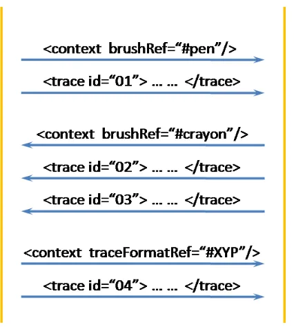
Figure 4.2: Example of InkML Streaming style
4.2.2
SketchML to Streaming InkML
InkML streaming delivers strokes in sequential time order. Compared with InkML archiving, contextual information are inserted into the stream of the strokes, as needed, to provide interpretation. Changes to the current context are given by <context> elements. This corresponds to an event-driven model of ink genera-tion, where events which result in contextual changes map directly to elements in the markup. An example of the InkML streaming style is shown in Figure 4.2. In this example, the participant A first sends a context change event. It notifies the partici-pant B that the stroke “01” must be interpreted as a “pen” stroke. The participartici-pant B then sends another context change event followed by stroke “02” and stroke “03”. It specifies that both the strokes must be interpreted as “crayon” strokes. Later, the participant A switched trace format to “XYP”. It notifies the participant B that each ink point of the stroke “04” should be treated as (x, y, p) triplet, where the x and y are the position coordinates of the ink point, and the pis the pen tip pressure.
< shape id = " 5 a6b5e88 -5274 -404 e - abb2 -19 c 2 e 4 0 3 5 1 c 9 " type = " S u b S t r o k e " width = " 150 "
author = " 86 bf5a7b - b71b -4912 - a3aa - e 6 8 6 f 5 a b d f 1 b " height = " 1 " name = " stroke " / >
</ a n n o t a t i o n X M L >
< trace xml:id = " Trace2 " >
3305.0 9966.0 1 1 8 0 1 1 3 6 5 7 0 3 8
2 7 5 8 9 4 4 1 8 6 4 4 8 6 2 8 1 7 6 - 6 3 7 7 4 7 3 1 2 6 0 13 61 34 01 23.0 , 3330.0 9952.0 1 1 8 0 1 1 3 6 5 7 0 4 6
- 7 9 9 8 1 1 2 3 1 9 7 67 16 36 65 - 5 3 7 2 3 9 9 5 7 6 9 7 63 23 10 3 29.0 , ...
</ trace > </ t r a c e G r o u p >
Listing 4.3: Example of conversion from SketchML to InkML streaming style.
element must appear prior to the<traceGroup> element. An example of conversion from SketchML to InkML streaming style is shown in Listing 4.3.
Converting from SketchML to InkML streaming style is useful in that it allows SketchML data to be shared instantly as it was captured. This enables SketchML applications to be used in collaborative scenarios, such as classroom teaching, distance education, work-group meeting, and collaborative document annotation, where sketch data must be transmitted in real time and properly interpreted by other participants.
4.3
InkML to SketchML
4.5
Summary
Part II
Handwritten Mathematical
Symbols
In a variety of applications, such as handwritten mathematics and diagram labelling, it is common to have symbols of many different sizes in use and for the writing not to follow simple baselines. In order to understand the scale and relative positioning of individual characters, it is necessary to identify the location of certain expected fea-tures. These are typically identified by particular points in the symbols, for example, the baseline of a lower case “p” would be identified by the lowest part of the bowl, ignoring the descender. We investigate how to find these special points automatically so they may be used in a number of problems, such as improving two-dimensional mathematical recognition and in handwriting neatening, while preserving the origi-nal style. This chapter is based on the article “Determining Points on Handwritten Mathematical Symbols” [35] co-authored with Stephen M. Watt, that appeared in the proceedings of 2013 Conferences on Intelligent Computer Mathematics.
5.1
Introduction
5.2
Determining Points
In order to find the scale and offset of individual characters, it is necessary to identify the location of certain expected features which are typically defined by particular points. These particular points occur at different locations in different symbols, and the precise location can vary in different handwriting samples of the same symbol. For example, the baseline of lowercase “p” would be identified by the lowest part of the bowl, ignoring the descender. In contrast, the baseline of lowercase “k” would be identified by the toes. In this chapter we refer to a point such as this, that deter-mines the height of a metric line, as a determining point. Knowing the determining points of each symbol can help us solve a number of problems. For example, one can use the determining points to improve two-dimensional mathematical recogni-tion. By comparing the baseline locations and the sizes of adjacent symbols, one can identify subscripts and superscripts (e.g. S2, S2,S2) with more confidence. Another application is in handwriting neatening. Since handwritten symbols often come with variations in alignment and size, certain transformations based on determining points can be applied to obtain normalized samples while preserving the original writing style.
5.3
Challenges
5.4
Previous Work
We are interested in the problem of how to automatically find determining points of handwritten mathematical symbols and to use them in a variety of problems. Consid-erable related work has been conducted, some of which we highlight here. Pechwitz and M¨argner [36] proposed an algorithm that can find determining points from sym-bol skeleton approximated by piecewise linear curve. However, these determining points are only useful in detecting baseline locations. In 2010, Infante Vel´azquez [37] developed an annotation tool to record determining points manually for handwritten characters represented in InkML. The determining points were later used to neaten new handwriting, making it uniform in size, alignment and slant while preserving writers’ particular writing styles. However, this tool recorded each determining point with absolute coordinates and was therefore subject to device resolution and vari-ations in style. As device resolution may vary among different vendors and over generations of technology, this approach is not device-independent. Similar problems exist in [38]. In addition, Zanibbi et al. [39] proposed a technique to automatically improve the legibility of handwriting by gradually translating and scaling individual symbol to closely approximate their relative positions and sizes in a corresponding typeset version. This technique detects baseline locations by comparing symbols’ bounding boxes, which leads to troubles with vertical placement and scale. For ex-ample, it fails to distinguish between “x2” and “x2
pro-Figure 5.1: An example to illustrate the concepts of metric lines.
posed a method to find determining points in handwritten Arabic characters. The method consisted of two stages. In the first stage, the raw input data were converted to a standard format using smoothing, normalization and interpolation techniques. In the second stage, each stroke of input characters was split into several pieces. The method calculated the local maximum and minimum of each piece and recorded them as determining points. However, this method is not optimal as it requires extra effort to split strokes and may generate undesired determining points that lack meaning.
5.5
Objectives
the average symbols. This reduces cost significantly. Furthermore, the algorithm is device-independent as all symbols are represented in the functional space, which is robust against changes in device resolution.
The remainder of this chapter is organized as follows. Section 5.6 discusses sev-eral types of determining points that are useful in finding symbol alignment lines. In Section 5.7, we present the algorithm that can identify determining points in hand-written mathematical symbols automatically. Section 5.8 evaluates the performance of the algorithm. We then investigate the possible use of the algorithm in a number of problems in Section 5.9. Section 5.10 concludes the chapter.
5.6
Handwriting Metrics
(a) (b)
Figure 5.3: X line and X height with (a) one, and (b) multiple determining points.
Baseline
Most scripts share the notion ofbaseline. It is a guide line for writing so that adjacent symbols can retain their horizontal alignment. It is also used as the reference to obtain other metrics such as x height, ascender height, etc. While some symbols such as lower case “p” may extend below the baseline, it serves as the imaginary base for most symbols. Figure 5.2 shows examples of baselines and their determining points. As shown in Figure 5.2(b), the three legs of the lowercase “m” are not completely aligned. In such case, multiple determining points are identified and the location of the baseline may be determined by the averagey value of all the determining points.
X Line and Height
The x line falls at the top of most lowercase symbols, such as “a” and “y”, and is located over the baseline. Some symbols may extend above the x line, such as “h” where the x line is located at the top of the shoulder. The x height is the distance between the baseline and the x line. Figure 5.3 shows an example of x line and associated determining points. Certain symbols, such as lowercase “x”, may have multiple determining points to define the x line. In such a case, the location of the x line is determined by the average of their y values.
Ascender Line and Height
is determined by the height of the ascenders. The ascender height is the distance between the baseline and the ascender line. Figure 5.4 shows an example of an ascender line and ascender height. The location of the ascender line is determined by the determining point shown in red. In the case that there are multiple determining points, the location of the ascender line is given by the average y value of all the relevant determining points.
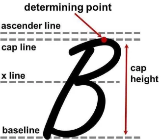
Cap Line and Height
The cap line is usually located below the ascender line, but is not limited to that position. It is used to measure the height of uppercase symbols, which is the distance between the baseline and the cap line. Figure 5.5 shows an example of cap line and
cap height. The location of the cap line is determined by the determining point shown in red. In the case that there are multiple determining points, the location of the cap line is determined by the average y value of all the determining points.
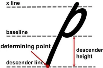
Descender Line and Height
Figure 5.6: Descender line and height Figure 5.7: Slant (θ) and width
Slant and Width
In some handwriting styles, symbols are written with inclination either to the left or to the right. The degree of inclination is referred to as the slant. The width of a symbol is given by the horizontal distance from the left-bounding and right-bounding lines with the given slant. Figure 5.7 shows an example of symbol width and slant.
5.7
Algorithms
In this section, we present an algorithm to find automatically the determining points for newly written symbols. The algorithm derives determining points for a new symbol from the known determining points of an annotated average symbol of the same type.
Average Symbols
We classify symbols so that symbols that are written the same way and could be interpreted the same way are in the same class. So, for example, there may be several classes for the numeral “8”, depending on whether the symbol is written with one continuous stroke or two separate strokes, which stroke is written first and the direction of writing. On the other hand, a Latin letter “O” and the numeral “0” could belong to the same class.
points of the same class falls within that class. It is therefore meaningful to compute the average of a set of known samples for a class as the average point in the function space
¯
C =
n
X
i=1 Ci/n,
wherenis the number of the samples andCiis the coefficient vector for theithsample. Figure 5.8(a) shows a set of samples provided by different writers and Figure 5.8(b) shows the average symbol.
Deriving Determining Points from Average Symbols
Our algorithm is based on the observation that the average symbols typically look similar to the samples of the same class. Within a given class, the features present in one sample should be present in other samples and at a similar location. We can take the location to be the arc length along the ink trace to the defining point of the feature. We assume that, if two symbols are sufficiently similar, the locations of corresponding determining points will be similar (given by distance along the curve).
value Ki states whether the metric line is given by a local minimum or local maximum atyA(si).
S, the coefficient vector for the input sample whose determining points are to be found.
Output: DS = [(ℓ1, T1, K1), . . . ,(ℓn, Tn, Kn)], giving the locations, ℓi, and types of the determining points ofS.
1. Let xA(s),yA(s), xS(s),yS(s) be the coordinate functions of the symbols given by A and S. 2. for i∈1..n do
if Ki =max then f ←− −yS
if Ki =min then f ←−+yS
ℓi ←−s such thatf(s) is minimized near si.
Note this is the local minimum of a real univariate polynomial and any standard method may be used. For example, we use Newton’s method to solve f′(s) = 0 with initial point s=s
i.
3. Return[(ℓ1, T1, K1), . . . ,(ℓn, Tn, Kn)]
For each determining point of the annotated sample, we guess that the correspond-ing determincorrespond-ing point on the new sample will be near the same arc length location. So we take the point at that location in the new sample and follow the trace upward or downward, depending on whether that determining point is supposed to be at a local minimum or local maximum. This can be easily done using a number of numerical methods. In our implementation, we applied Newton’s method to solve y′(s) = 0. A
formal algorithm is given in Algorithm 3.
(a) (b) (c) (d) (e)
Figure 5.10: Automatically finding determining points. (a) Average symbol “π”. (b-e) Determining points derived from the average symbol.
and 5.9(c2) show the determining points found at locations ℓi. Figure 5.10 shows several examples of determining points found for samples of “π”.
5.8
Experiments and Testing
We developed a software tool to annotate handwriting samples with their determining points. Figure 5.11 shows the user interface. By selecting a nearby location, the tool is able to find the target determining point automatically. The locations of all the metric lines discussed in Section 5.6 can be detected. Multiple determining points may exist for certain metrics lines. In such circumstances, the location of the corresponding metric line is determined by the average of the values given by all the determining points of that kind. Symbol slant can also be recorded by adjusting a spinner. Symbol width is automatically detected with slant considered.
hand-Figure 5.11: Software tool to annotate a symbol with determining points.
dif-ferent orders), a total of 382 classes were examined. We first computed the average symbol for each class, in which determining points were identified using the software tool shown in Figure 5.11.
We then computed determining points for all the samples using Algorithm 3. The number of determining points varied from 2 to 5, according to the sample. If any of the determining points were mis-positioned, we considered it as incorrect. We chose up to 30 samples randomly from each class and examined their correctness visually. In total, we examined 8119 samples, of which 421 samples have at least one mis-positioned determining point. This gave a measured error rate of 5.2%.
We found the error was introduced mainly from two sources. The first was mis-classified samples in the original data set. These were either mis-labelled (e.g. “e” of style 1, instead of “e” of style 2), or had strokes given in a different order from the usual. In this latter case, we have the option of defining a new style or normalizing the order of the strokes. The second source was that some samples are significantly different from the average symbol. As a result, the determining points in the average symbol may not be mapped correctly to those dissimilar samples.
As misclassified samples were errors in the training data, rather than errors by the algorithm, we excluded those samples from the experiment. We further added 39 new classes (giving 421 classes in total) to split out those samples with different stroke orders. After these corrections, the measured error rate decreased to 2.0% (9593 samples reviewed, of which 189 samples had at least one mis-positioned determining point).
(d) (e) (f)
Figure 5.13: Success in 5 steps: (a) average symbol (b) step 1 (c) step 2 (d) step 3 (e) step 4 (f) step 5 = target.
test sample in a multi-step method. Recall that, in the function space, a line from the average symbol to the test sample lies entirely within the class. By dividing this line into several equal steps, we may apply Algorithm 3 several times to follow the determining points through the homotopy. If ¯C is the average symbol for the class and Ctarg is the input sample, then the line joining the two points in the function space is given byC(t) = (1−t) ¯C+tCtarg, withtranging from 0 to 1. The determining points should move smoothly as the character is deformed by the homotopy, and we can choose a step size. Figure 5.12 shows an example where Algorithm 3 fails to identify one of the determining points when applied naively. However, when applied in a 5 step homotopy, it succeeded, as shown in Figure 5.13.
Figure 5.14: Error rates of the multi-step method on 9593 samples.
(a) (b) (c) (d)
Figure 5.15: Multi-step failures: (a) Average, (b) target. (c) Average, (d) target.