Article
1
Towards Sensor Reliability Using Internet-of-Things
2
LiDAR Data in a Cyber-Physical System
3
Fernando Castaño1,*, Alberto Villalonga1, Rodolfo E. Haber 1, Joanna Kossakowska 2 and
4
Stanisław Strzelczak 2
5
1 Centre for Automation and Robotics (CSIC –UPM), Spanish National Research Council, Arganda del Rey,
6
Madrid, 28500, Spain; [email protected]
7
2 Faculty of Production Engineering, Warsaw University of Technology, Warsaw, Poland;
8
9
* Correspondence: [email protected]; Tel.: +34-918-70-50 (F.C.)
10
11
Abstract: Currently, the most important challenge in any assessment of state-of-the-art sensor
12
technology and its reliability is to achieve road traffic safety targets. The research reported in this
13
paper is focused on the design of a procedure for evaluating the reliability of Internet-of-Things
14
(IoT) sensors and the use of a Cyber-Physical System (CPS) for the implementation of that evaluation
15
procedure to gauge reliability. An important requirement for the generation of real critical situations
16
under safety conditions is the capability of managing a co-simulation environment, in which both
17
real and virtual data sensory information can be processed. An IoT case study that consists of a
18
LiDAR-based collaborative map is then proposed, in which both real and virtual computing nodes
19
with their corresponding sensors exchange information. Specifically, the sensor chosen for this
20
study is a Ibeo Lux 4-layer LiDAR sensor with IoT added capabilities. Implementation is through
21
an artificial-intelligence-based modeling library for sensor data-prediction error, at a local level, and
22
a self-learning-based decision-making model supported on a Q-learning method, at a global level.
23
Its aim is to determine the best model behavior and to trigger the updating procedure, if required.
24
Finally, an experimental evaluation of this framework is also performed using simulated and real
25
data.
26
Keywords: Cyber-Physical Systems; reliability assessment; Internet-of-Things; LiDAR sensor;
27
driving assistance; obstacle recognition; reinforcement learning; Artificial Intelligence-based
28
modelling.
29
30
1. Introduction
31
Nowadays, knowledge of the most appropriate sensor operating conditions and fault detection
32
systems are among the cornerstones of scientific and technical studies for automated systems [1].
33
These are based upon on-line monitoring processes and additional comprehensive interpretation of
34
sensor data, by assessing sensor reliability. Sensors are driving the rapid growth of Cyber-Physical
35
Systems (CPSs) and the Internet of Things (IoT). Both paradigms are behind the next generation of
36
sensor networks and unpredictable future applications, meaning that sensor reliability has become
37
one of the most important and desirable performance indicators in the design, implementation, and
38
deployment of future sensor networks [2].
39
An important reliability-related issue to be detected in autonomous systems is the failure of one
40
network element, in order to self-correct problems such as lost data packages, and data collision,
41
among others [3]. One possible solution is to build real-time prediction models that maximize
42
robustness and lifetime [4]. There are, in fact, several methods for the evaluation of sensor reliability.
43
Each component that constitutes reliability or that might affect it can be assessed individually and as
44
a whole, through a total error band figure. There are important features to be considered such as
45
sensitivity, range, precision, resolution, accuracy, offset, linearity, dynamic linearity, hysteresis and
46
response time. Evaluating sensor reliability includes probabilistic and statistical data that increase
47
estimation reliability [5]. Evidence theory can be used, such as the Dempster-Shafer theory of belief
48
functions. Quantifying reliability implies predictions concerning sensor lifetime and failure
49
probability. Reliability can therefore be based on both statistical and Artificial Intelligence (AI)
50
models. Suitable probability functions must be defined, which will be used to calculate the future
51
behavior of devices, based either on carefully controlled laboratory experiments or on thorough
52
failure analysis while in use. A typical product will be liable to various failure modes that change
53
over time in a characteristic manner, so that the probability functions are themselves time dependent.
54
The most widely used techniques for modelling predictions concerning product lifetime and
55
failure probability are probabilistic methods. Probabilistic methods for uncertain reasoning represent
56
another group of techniques. Probability theory predicts events from a state of partial knowledge,
57
while Fuzzy-Logic models are applied to situations with intrinsic vagueness and uncertainty.
58
However, the prediction techniques are hardly limited to those mentioned above. Several
59
clustering techniques such as nearest neighbor methods have been explored, in order to enable
self-60
detection and self-correction capabilities [6]. Other capabilities to be considered from the perspective
61
of reliability are self-adaptation and self-organization by embedding artificial neural networks
62
(ANNs) in CPSs [7]. Efficient performance of multiple sensors and their online monitoring and
self-63
correction procedures, through the application of machine learning (ML) such as Support Vector
64
Machines (SVM) and ANNs, are very important for the reduction of maintenance costs, risk
65
minimization associated with uncalibrated and faulty sensors, increased instrument reliability and,
66
consequently, extended equipment life [8, 9].
67
With the aim of guaranteeing certain safety and security conditions in some critical applications,
68
the verification of sensory data and subsequent data evaluation are described in this paper through
69
the simulation of virtual and real scenarios, as well as frameworks that properly combine both
70
scenarios.
71
A reliability assessment procedure is therefore described in this paper that is applicable to data
72
captured by IoT LiDAR sensors in automotive applications: LiDAR self-testing methodology. The
73
reliability analysis is based on the paradigm of cyber-physical systems (CPS) by distributing nodes
74
locally and globally, as will be explained later on. Each computing node has data-processing methods
75
and machine-learning models for reliability prediction. In addition, a run-time self-learning and
76
decision-making model runs within a global node, in order to determine the best model and the
77
model updating mechanism on request.
78
The paper will be organized into five sections. Following this introduction, the second section will
79
present a state-of-art review of the CPS-based reliability concept for sensor system reliability using
80
AI methods. Subsequently, the specifications and the requirements obtained from the review of CPS
81
reliability frameworks will be summarized in section 3. A particular implementation of a CPS-based
82
co-simulation framework will also be proposed in this section. In addition, a case study for the
83
evaluation of an IoT sensor network using a CPS-based co-simulation framework approach will be
84
described in section 4. In that section, the experimental results and a discussion relating to a
85
comparative study will also be addressed. Finally, the conclusions and future research steps will be
86
presented in section 5.
87
2. CPS-based reliability approach
88
The truly challenging aspects of sensor network reliability and its evaluation have yet to prompt
89
an exhaustive exploration and evaluation of sensory data under critical conditions. A gap that is
90
addressed in this study through sensors incorporated in a CPS.
91
92
93
2.1. Sensor reliability assesment
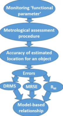
One approach to sensor reliability in automotive applications is to design a model-based
95
relationship between ‘model parameters’. Those parameters can be derived from process monitors
96
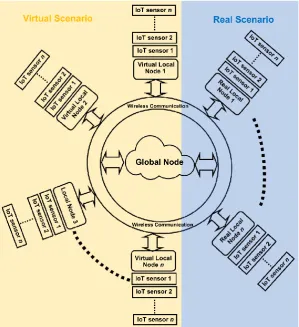
while ‘functional parameters’ refer to both the sensor characteristics and sensor lifetime, as well as
97
cost aspects due to process yields (see Figure 1).
98
With the aim of increasing the reliability of data collected by LIDAR, metrological assessment
99
procedures must also be applied. Linear interpolation of measurements from three detectors
100
arranged in series is a time-saving procedure for processing and reducing LIDAR data [10].
101
102
103
Figure 1. Procedure for sensor reliability assessment using model-based relationship between sensor
104
data and key performance indices.
105
All the major sources of potential error that could influence point positioning accuracy have to
106
be considered in the analytical derivations, in order to determine the reliability of achievable point
107
positioning accuracy of LiDAR systems. Csanyi, May and Toth provided some of the random errors
108
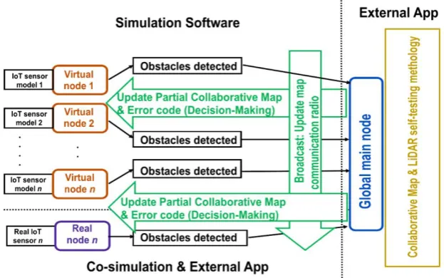
that will be considered [11]. They also provided some formulas for point positioning accuracy that
109
were derived from the LiDAR equation, via rigorous error propagation:
110
111
𝑟𝑀 = 𝑟𝑀,𝐼𝑁𝑆+ 𝑅𝐼𝑁𝑆𝑀 (𝑅𝐿𝐼𝑁𝑆∙ 𝑟𝐿+ 𝑏𝐼𝑁𝑆) (1)
112
where, 𝑟𝑀 represents the 3D coordinates of an object point in the mapping frame; 𝑟𝑀,𝐼𝑁𝑆 represents
113
time dependent 3D INS coordinates in the mapping frame, provided by GPS/INS; 𝑅𝐼𝑁𝑆𝑀 is the time
114
dependent rotation matrix between the INS body and the mapping frame; 𝑅𝐿𝐼𝑁𝑆 is the boresight
115
matrix between the laser frame and the INS body frame; 𝑟𝐿represents the 3D object coordinates in
116
the laser frame; and, 𝑏𝐼𝑁𝑆 is the boresight offset vector.
117
In addition, the calculation of the accuracy of the estimated location for an object using the
118
LiDAR sensor can be performed by other key performance indices. For example, the use of the
119
Distance Root Mean Squared (DRMS) measure for the data that are tracked on the x-y plane (2D) and
120
the Mean Radial Spherical Error (MRSE) measure for the data that are tracked in the x–y–z space (3D)
121
were reported in [12, 13]. Using derivable error formulas, any given random error and scan angle in
122
the LiDAR range can be modelled and simulated. By doing so, the factors affecting LiDAR system
123
accuracy can be analyzed [14].
124
2.2. Statistical and Artificial Intelligence-based methods
125
Bayesian and Hidden Markov models are the most widely applied for reliability assessment
126
under fuzzy environments [15, 16]. A Bayesian network is a directed acyclic graph consisting of a set
127
of nodes, representing random variables and a set of directed edges, representing their conditional
dependencies. The dependencies in a Bayesian network can be adaptively determined from a dataset
129
through a learning process. The objective of this training is to induce the network with the best
130
description of the probability distribution over the dataset and can be categorized as an unsupervised
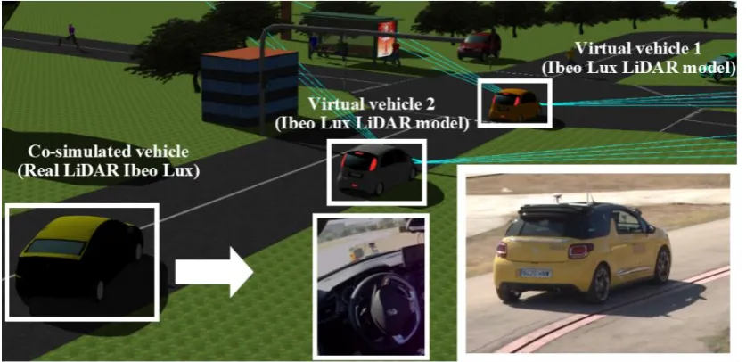
131
learning method, because the attribute values are not supplied in the dataset [17].
132
In addition to those probabilistic methods, new tools are reported in the literature, highlighting
133
theuse of Artificial Intelligence (AI) techniques and in particular, Machine Learning (ML), to solve
134
complex situations [18]. AI techniques also provide cognitive abilities, so that performance may be
135
improved by increasing network life-time and reliability [19]. Some of those techniques are ANN and
136
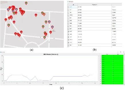
fuzzy inference system [20, 21]. Zhang et al. proposed a soft-computing system based on Genetic
137
Algorithm-Support Vector Regression (GA-SVR), in order to facilitate the reliability and survivability
138
of the Structural Health Monitoring (SHM) system faced, for example, with an invalid fiber link in
139
the sensor network [22].
140
3. CPS-based co-simulation framework
141
Some factors that can affect CPS reliability are component failure, environmental effects, task
142
changes, and network update. A strategy for testing the reliability of CPSs and for their evaluation is
143
proposed in [23] by analyzing both the internal and the external factors that influence their reliability.
144
One solution could be to evaluate each element that constitutes the system: testing hardware,
145
software, and architecture, as well as performance reliability including service reliability, cyber
146
security reliability, resilience & elasticity reliability, and vulnerability reliability.
147
Behavioral simulations of CPS and IoT assume importance as a method to analyze reliability,
148
because the mathematical modeling of those factors is so difficult [24]. Those simulations are based
149
on addressing four main topics: node localization, energy management, network multi-objective
150
optimization, and self-capabilities approach [25, 26].
151
While the reliability evaluation of physical systems is well-understood and has been extensively
152
studied, the reliability evaluation of a CPS is of greater complexity, because software systems will not
153
degrade and follow a well-defined failure model in the same way as physical systems. An evaluation
154
framework is therefore necessary, in order to assess the CPSs. A framework for CPS reliability
155
analysis that includes reliability-based runtime reconfiguration is proposed in [27]. This framework
156
is codified in a domain-specific modelling language that provides details on operational constraints
157
and dependences.
158
However, domain-specific modelling-based analysis is, in many cases, unable to compute
159
reliability functions efficiently (e.g. in terms of failure distributions) for complex systems. To do so, a
160
frequency-domain reliability analysis framework of transportation CPSs was described in [28]. The
161
advantage of that method is its capability to capture higher-order moments of the system
162
characteristics, its scalability for the analysis of the reliability of complex systems, and efficient
163
calculations.
164
In addition, it is important to consider the evaluation of other aspects of the CPS, such as safety
165
and particularly security, different aspects of which have been focused upon over the past few years.
166
Therefore, the design of the CPS framework must address those aspects at three levels: security
167
objectives, security approaches and security in specific applications [29]. However, not only must the
168
cyber part be secured, but also the physical part of possible threats. A multi-cyber (computational
169
unit) framework was compared with traditional models to improve the availability of the CPS based
170
on the Markov model. It was efficiently evaluated, in terms of availability, downtime, downtime
171
costs, and the reliability of the CPS framework [30].
172
Finally, another work considered an Internet-based computing platform in the form of a global
173
computing node. In [31], a new cloud security management framework was introduced, based on
174
improving collaboration between cloud providers, service providers, and service consumers for the
175
management of cloud platform security and the hosting services. In addition, although in some
176
applications this will not be possible, it is important to consider the possibility of introducing the
177
human factor in the reliability analysis procedure. A human-interactive Hardware-In-the-Loop
Simulation (HILS) framework for CPS was developed in [32] to support reliability and reusability in
179
a fully distributed operating environment.
180
3.1. CPS-based co-simulation framework proposed
181
Based on the above contributions and considering the initial list of requirements from the
182
previous section for the deployment of an IoT sensor network, a CPS-based co-simulation framework
183
is proposed where an IoT sensor network will supply physical data and (local and global) computing
184
nodes for processing the sensory data.
185
3.1.1. Conceptual Scheme
186
In addition, the IoT sensor network has a global or main node composed of a knowledge
187
database, a Q-learning method for decision-making and an AI-based model library. During the
188
simulation and the real running, a decision-making module will decide which specific model is the
189
best in the current instant, taking into account the data received by all nodes that make up the
190
network.
191
The functionalities are distributed in different nodes, both virtual and real, according to their
192
functions. The distributed virtual or real nodes manage the capture of sensory data and run the error
193
prediction calculation with the required accuracy, while the global or main node incorporates the
194
runtime model that is generated, the library, and the knowledge database (see Figure 2).
195
196
197
Figure 2. General scheme of the CPS-based co-simulation framework with virtual and real computing
198
nodes and IoT sensor network.
199
The IoT sensors should be able to establish reliable and accurate wireless communications,
200
ensuring that all the intrinsic challenges in an IoT network and in the different CPSs can be solved. It
201
is achieved through the implementation of the architecture that is represented in Figure 2: a network
of n nodes, each node having n IoT sensors. In addition, the computing nodes must communicate
203
with each other and with their corresponding global node.
204
3.1.2. Procedure description
205
The framework is designed with the condition that both the real and the virtual (local)
206
computing nodes must operate in parallel with the global computing node [33]. Data exchange
207
between the different nodes takes place in two different ways. On the one hand, data exchange
208
between local nodes is produced in both the virtual (3D model simulation tool) and the real scenario.
209
On the other hand, there is the data exchange between different local nodes and the global node using
210
the 802.11p wireless communication protocol.
211
There is therefore interaction between the software for both the simulated and the real
212
environments, and external applications that are running in the main node. Figure 3 shows the
213
schematic diagram of the exchange of information or messages within the co-simulation framework.
214
215
216
Figure 3. Conceptual flowchart showing the operation of a reliability co-simulation framework with
217
CPS computing nodes and IoT sensors.
218
In the particular implementation that is described more accurately in the following section, there
219
is a wireless exchange of messages between different nodes using the 802.11p communication
220
protocol in the following way. First, the local nodes with their IoT sensors detect different objects and
221
their respective properties. Secondly, this information is shared on the network through a broadcast
222
process.
223
4. IoT LiDAR-based collaborative mapping – A case study
224
The IoT sensor network chosen to evaluate the CPS-based co-simulation framework is composed
225
of virtual and real LiDAR sensors [34]. An Ibeo Lux LiDAR 4-layer sensor was used with the
226
following specifications: horizontal field of 120 deg, horizontal step of 0.125 deg., vertical field of 3.2
227
deg., vertical step of 0.8 deg., range of 200 m, and an update frequency of 12.5 Hz. As previously
228
mentioned, the sensor network to be evaluated is composed of IoT sensors. The sensor network
229
therefore has IoT capabilities connected to its computing nodes. These nodes are on-board computers
230
integrated in an autonomous vehicle with a wireless communication interface between them.
231
The particular implementation of the CPS-based co-simulation framework, the LiDAR-based
232
collaborative map, is based on a co-simulation framework between two different software systems,
233
both for the simulated part, designed in [35]. However, the contribution of this study is to include the
234
real part in the co-simulation framework. This framework consists mainly of a computer-aided
235
system to enable efficient interaction between the virtual scenario with virtual nodes setting in the
236
Webots automobile simulation tool 8.6 [36] and an external application development for the
computing nodes in the real scenario. The scenario in this particular case, in which the vehicles are
238
represented as nodes, is as follows. A real vehicle (in a real scenario) and three virtual vehicles in the
239
simulated scenario are detecting obstacles. Both kinds of vehicles share the position, object type and
240
size of the obstacles (e.g., pedestrian, trees on the road and another vehicle). This is possible thanks
241
to the IoT LiDAR network using an IoT obstacle detection application (see section 4.1), created in run
242
time. Figure 4 shows the detailed diagram of the implementation of the LiDAR-based collaborative
243
map using the CPS-based framework approach.
244
245
246
Figure 4. Detailed diagram of the implementation of the LiDAR-based collaborative map approached
247
through a CPS-based co-simulation framework.
248
As previously mentioned above, the exchange of information packets between the local nodes
249
with the main or global node is possible; thanks to the use of a communication protocol using a UDP
250
(User Datagram Protocol) as the transport layer and a Wi-Fi 802.11p as the physical layer. The
251
visualization of the co-simulated vehicle (real node) in the 3D virtual scenario in the Webots
252
simulation tool is also possible. An example of the execution of the co-simulation architecture can be
253
seen in Figure 5.
254
255
256
Figure 5. Data interchange between LiDAR sensors in (virtual and real) driving assistance scenarios
257
in Webots for automobiles.
In addition, another application implemented in the IoT LiDAR-based collaborative map is the
259
LiDAR self-testing methodology incorporated in each local computing node (autonomous vehicle),
260
in order to evaluate the reliability of each IoT sensor in the network (section 4.2).
261
4.1 Obstacle detection in the IoT application
262
This framework is implemented in an external application; a development in Qt 5.10, that
263
consists of an illustrated map updated in run time (see Figure 6 (a)) and a database with the
264
information on both the virtual and the real objects that are detected (see Figure (b)). The information
265
contains the position, object type, and size of the obstacles, to improve on the security/safety of the
266
object detection process with a single sensor.
267
268
(a) (b)
(c)
Figure 6. (a) Collaborative mapping; (b) obstacles detected database; (c) LiDAR data for run-time
269
accuracy error detection.
270
Figure 6 depicts the visual interface of the framework that has been developed. Specifically, the
271
collaborative map is globally updated in the main computing node. A partial area of this updated
272
map can also be sent at the request of a local node. A set of computational procedures is in charge of
273
adapting and transferring sensory information from Webots, virtual nodes with the Ibeo Lux sensor
274
model, and the real node, real vehicles with the real Ibeo Lux sensor; and vice versa.
275
4.2. LiDAR selft-testing application
276
The external application also includes a LiDAR data self-testing methodology using the
AI-277
based error-prediction models. Figure 6 (c) shows the graphical interface that represents the
278
estimated error with regard to time on the left-hand side. However, on the right-hand side the
279
admissible error threshold is observed, which if exceeded, must be requested to make decisions over
280
the best performance of each model at any given time. Specifically, the results are focused on showing
281
the improved performance of the IoT sensor network composed of each CPS element with each
LiDAR sensor plus added IoT capabilities. To do so, a reliability prediction model dedicated to
283
obtaining the accuracy error in obstacle detection is incorporated in each computing node.
284
4.2.1. Reliability prediction models
285
A reliability model was generated for each IoT LiDAR sensor, both virtual and real, that
286
predicted the accuracy error for obstacle detection. The steps to follow for the determination of those
287
models were extracted from the methodology described in [37, 38], with a set of different training
288
data. In this study, a model-based procedure was used with a point-cloud clustering technique, in
289
this case Density-Based Spatial Clustering of Applications with Noise (DBSCAN) [39]. In addition,
290
an error-based prediction model library was described, highlighting AI-based model techniques,
291
such as, Multilayer Perceptron Neural Network (MLP), k-Nearest Neighbors (k-NN), and Linear
292
Regression (LR). A difference in the particular implementation described in this paper is that, while
293
k-NN, MLP and LR were maintained, SVM was added as a new technique to the AI-based library
294
[40-42].
295
4.2.2. Model parametrization and validation
296
With the aim of determining which model training strategy based on AI provides the best
297
reliability prediction model, an experimental validation was performed. The training dataset was
298
composed of 998 scenes for the model training and 250 scenes for the model validation. All of them
299
were obtained from a simulation procedure. The data input consisted of geospatial statistics [13, 43]
300
which were extracted from the point cloud supplied by the LiDAR sensor, so that the models could
301
generate the figures of merit in terms of accuracy error: DRMS and MRSE.
302
The four AI-based strategies that were considered are as follows. First, a multilayer perceptron
303
neural network with backpropagation (MLP) with two hidden layers, each with five neurons and
304
sigmoid activation functions, and an output layer with a lineal activation function, two neurons, and
305
5000 epochs. The initial value of the learning rate (μ) was 10-3 with a decrease factor ratio of 10-1, an
306
increase factor ratio of 10, and a maximum μ value of 1010. The minimum performance gradient was
307
10-7. The training process stop criteria were as follows: the maximum number of epochs (repetitions);
308
goal performance minimization; the performance gradient below a minimum gradient; or, a
value309
in excess of the maximum value. The second modeling technique was k-nearest neighbors (k-NN),
310
with k = 5 and using Euclidean distance as the distance function. The third was a lineal regression
311
that was also obtained by minimizing the sum of squared differences between the predicted and the
312
observed values. Finally, a support vector machine model was fitted by means of data
313
standardization and the radial basis function kernel.
314
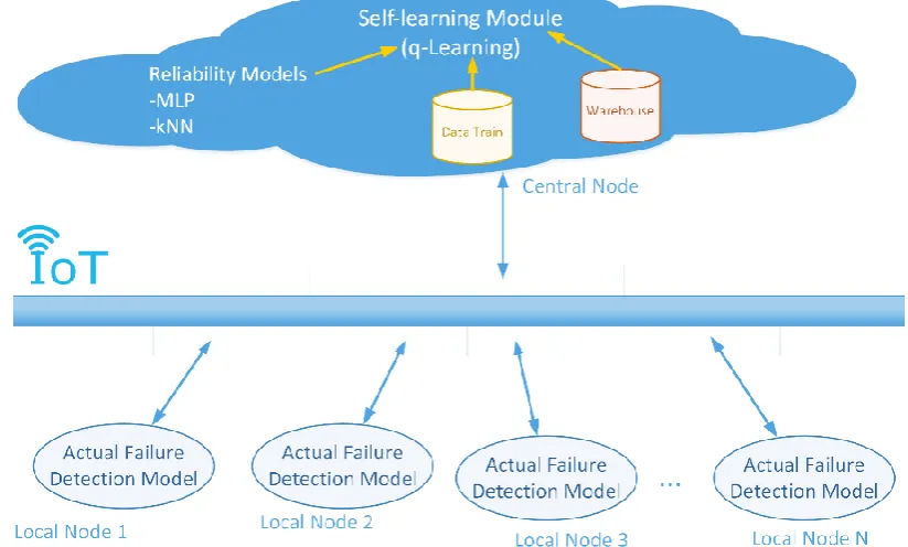
4.2.3. Self-learning-based decision-making. Q-learning algorithm
315
The global or main computing node executes several parallel procedures in a specific
self-316
learning module that uses a Q-learning algorithm. On the one hand, a dataset for training by default
317
is present in the global node. On the other hand, a knowledge database (warehouse) is also included,
318
which can be updated in run time with the data provided by each local node. It sets up the
self-319
learning strategy that is run, in order to analyze the best model behavior, when new traffic situations
320
are generated providing new point clouds (environment information).
321
The local node, also in parallel, simulates the reliability model and when an error is admissible
322
the threshold will exceed 20% in one the figures of merits (DRMS or MRSE), which will mean that
323
the current model is failing. A request is therefore made to the global module to establish whether
324
there is a model that is working better. The decision to select the best prediction model included in
325
the library is taken by the self-learning decision-making at each instant, according to the
326
generalization capability and the accuracy of the model. The particular performance metrics for each
327
are R2 and RAE, respectively. In summary, based on this continuous information flow and the
328
previous prediction results (knowledge database), when a request from one of the local nodes is
received and a new best model behavior is detected, the current error prediction model is then
330
commuted, between MLP and k-NN, and vice versa.
331
332
333
Figure 9. Flow diagram between the global node (self-learning module), IoT network, and local
334
nodes (actual failure detection model).
335
5. Experimental results
336
5.1. Reliability model-based validation
337
Table 1. Key performance indices based on plane (DMRS) & space (MRSE) figure of merits.
338
Model MAE RMSE RAE RRSE R
2
DMRS MRSE DMRS MRSE DMRS MRSE DMRS MRSE DMRS MRSE
MLP 0.0046 0.0035 1.275 1.270 0.187 0.188 0.395 0.392 0.933 0.933
kNN 0.002 0.0002 1.014 1.010 0.114 0.114 0.371 0.365 0.963 0.961
LR 0.6781 0.6530 2.305 2.285 0.701 0.695 0.782 0.788 0.434 0.435
SVM 0.4735 0.4740 2.072 2.065 0.442 0.447 0.773 0.773 0.692 0.684
339
Table 1 shows the evaluation results obtained during the initial validation of each reliability
340
model. Five error-based performance indices and two classification criteria were considered in the
341
validation process: Mean Absolute Error (MAE); Root Mean Squared Error (RMSE); Relative
342
Absolute Error (RAE); Root Relative Squared Error (RRSE); and, the coefficient of determination (R2).
343
Only, the models generated with k-NN and MLP returned R2 results higher than 90%.
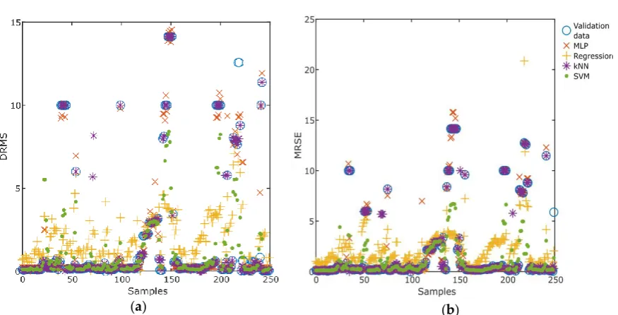
(a) (b)
Figure 7. Behavior representation of LiDAR error on the plane for each model with regard to the
346
validation data.
347
Figure 7 illustrates the behavior representation of the LiDAR error on the plane (DRMS) for each
348
model (MLP, LN, KNN and SVM) with regard to the validation data. The AI-based modeling
349
techniques that showed the best performing were MLP and KNN, according to the comparative study
350
of the four modelling strategies, with a percentage improved performance comparable to the other
351
two models of around 30%. Those model types will be chosen for the validation of the
decision-352
making module.
353
5.1. Self-learning for decision-making evaluation
354
Finally, a simulation in order to determine the quality of the Q-learning method in the automatic
355
selection of the best prediction model was performed. The reward function is chosen for setting the
356
best possible Q-value in 100 different scenes. Therefore, the function to update the Q-values is [44]:
357
358
(
)
(
)
(
)
1 , , ( , )( 1 max 1, ( , ))
t t t t t t t t t t t t t t t
a A
Q+ s a Q s a s a R+ Q s+ a Q s a
= + + − (2)
where, st is the state in time t; at is the action taken in time t; R(t+1) is the reward received after
359
performing action at; t is the learning rate; and, is the discount factor which trades off the
360
importance of sooner-versus-later rewards. Table 2 lists the error reward matrix based on knowledge
361
of the behavior of those prediction models.
362
363
Table 2. Q-learning reward matrix for error admissible threshold.
364
R2 RAE
0 – 10% 10 -20% 20 – 40% 40 – 70% > 70%
90 – 100% 1 0.9 0.8 0.5 0.2
80 – 90% 0.85 0.8 0.65 0.4 0.15
70 – 80% 0.7 0.6 0.5 0.3 0.1
30 – 60% 0.5 0.4 0.3 0.2 0.05
0 – 30% 0.3 0.2 0.15 0.1 0.01
365
366
The decision-making was based on two of the main performance indexes of model quality. First,
367
generalization capacity of the model. The Relative Absolute Error (RAE), which is a measure of model
369
accuracy, was the second parameter.
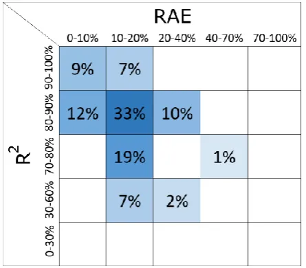
370
Figure 9 shows the Q-learning classification error matrix. As previously shown, the best model
371
had a RAE between 0 and 20% and a R2 above 80% in 61% of the scenarios. The system was able to
372
guarantee models with a greater capability of generalization in 71% of the scenarios, based on a
373
coefficient of determination that was over 80%. In total, reliability can be predicted with an RAE of
374
less than 40% and an R2 of over 70% in 90% of the scenarios, which demonstrates the quality of the
375
models. The models presented a low generalization, with a coefficient of determination of less than
376
70% in only 9% of the scenarios and a RAE greater than 40% in only 1%. Therefore, the Q-learning
377
method that evaluates reliability on the basis of the prediction error model at each instant worked
378
appropriately when determining the best model that represented the LiDAR performance to a high
379
degree of accuracy and that guaranteed the required levels of safety and reliability for automotive
380
applications.
381
382
383
Figure 9. Q-learning classification error matrix.
384
5. Conclusions
385
A method and an accompanying procedure have been presented in this paper for evaluating the
386
reliability of IoT sensors in a CPS. A co-simulation platform has been designed for that purpose where
387
virtual and real sensors can interact during run time through different simulations under appropriate
388
safety conditions. The co-simulation framework was composed of distributed computing nodes
389
within an IoT network, at both global and local levels.
390
A case study that consists of a LiDAR-based collaborative map has been proposed, in order to
391
validate the CPS-based co-simulation framework. Real and virtual computing nodes with the
392
corresponding sensors shared the position, object type, and size of the obstacles, to improve the
393
security and safety of the autonomous driving when detecting objects with this framework in run
394
time. The assessment of the proposed method was divided into two parallel procedures. First, at local
395
level, each reliability model evaluated the condition of the IoT LiDAR sensor. Secondly, at a global
396
level, a self-learning strategy for decision-making determined the most appropriate behavior of
397
models in the reliability model library, also in run time. The Q-learning method was selected for this
398
unsupervised self-learning strategy.
399
The comparative study of four strategies (MLP. SVM, k-NN and linear regression) in the
400
reliability modelling library was then performed. In summary, the MLP and the k-NN methods
401
outperformed the other two strategies considered in this study. Based on the previous results, a final
402
experimental evaluation was presented, in order to determine the quality of the Q-learning method
403
for automatically selecting the best reliability model. A Q-learning method evaluated the reliability
404
models, in order to perform the analysis, in a simulation study with 100 different scenarios. Based on
this procedure and the prediction results of the Q-learning method, when a request from one of the
406
local nodes is received, a new model behavior is detected, and the current error prediction model is
407
then commuted. Overall, all the reliability models performed very well, according to their
408
generalization capability.
409
Therefore, the proposed CPS-based co-simulation framework has served to assess the
410
performance of the IoT LiDAR network very accurately, guaranteeing safety and reliability in this
411
autonomous driving case study. These promising results pave the way for future work that will
412
validate the proposed method under real autonomous driving conditions.
413
Author Contributions: R.E.H., J.K. and S.S reviewed all technical and scientific aspects of the article. A.V. and
414
F.C was in charge of the implementation of software application, the library models and the reinforcement
415
learning algorithm. F.C. and A.V. designed and implemented the scenario, the external application and the
416
LiDAR self-testing procedure, and drafted the paper.
417
Acknowledgments: This work was partially supported by the project Power2Power: Providing next-generation
418
silicon-based power solutions in transport and machinery for significant decarbonisation in the next decade,
419
funded by the Electronic Component Systems for European Leadership (ECSEL-JU) Joint Undertaking and the
420
Ministry of Science, Innovation and Universities (MICINN), under grant agreement No 826417. In addition, this
421
work was also funded by the Spanish Ministry of Science, Innovation and Universities through the project
422
COGDRIVE (DPI2017-86915-C3-1-R). Preparation of this publication was also partially co-financed by the Polish
423
National Agency for Academic Exchange (NAWA) through the project: “Industry 4.0 in Production and
424
Aeronautical Engineering (IPAE)”.
425
Conflicts of Interest: The authors declare no conflict of interest.
References
428
1. Beruvides, G.; Quiza, R.; Del Toro, R.; Haber, R. E., Sensoring systems and signal analysis to monitor
429
tool wear in microdrilling operations on a sintered tungsten-copper composite material. Sensors and
430
Actuators, A: Physical 2013, 199, 165-175.
431
2. Kabashkin, I.; Kundler, J., Reliability of Sensor Nodes in Wireless Sensor Networks of Cyber Physical
432
Systems. Procedia Computer Science 2017, 104, 380-384.
433
3. Godoy, J.; Pérez, J.; Onieva, E.; Villagrá, J.; Milanés, V.; Haber, R., A driverless vehicle demonstration
434
on motorways and in urban environments. Transport 2015, 30, (3), 253-263.
435
4. Hao, X.; Wang, L.; Yao, N.; Geng, D.; Chen, B., Topology control game algorithm based on Markov
436
lifetime prediction model for wireless sensor network. Ad Hoc Networks 2018, 78, 13-23.
437
5. Guo, H.; Shi, W.; Deng, Y., Evaluating Sensor Reliability in Classification Problems Based on Evidence
438
Theory. IEEE Transactions on Systems, Man, and Cybernetics, Part B (Cybernetics) 2006, 36, (5), 970-981.
439
6. Zhang, H.; Liu, J.; Pang, A.-C., A Bayesian network model for data losses and faults in medical body
440
sensor networks. Computer Networks 2018, 143, 166-175.
441
7. Serpen, G.; Li, J.; Liu, L., AI-WSN: Adaptive and Intelligent Wireless Sensor Network. Procedia Computer
442
Science 2013, 20, 406-413.
443
8. Nsabagwa, M.; Mugume, I.; Kasumba, R.; Muhumuza, J.; Byarugaba, S.; Tumwesigye, E.; Otim, J. S. In
444
Condition Monitoring and Reporting Framework for Wireless Sensor Network-based Automatic Weather
445
Stations, 2018 IST-Africa Week Conference (IST-Africa), 9-11 May 2018, 2018; 2018; pp Page 1 of 8-Page
446
8 of 8.
447
9. Chuan, Y.; Chen, L., The Application of Support Vector Machine in the Hysteresis Modeling of Silicon
448
Pressure Sensor. IEEE Sensors Journal 2011, 11, (9), 2022-2026.
449
10. Rodrigues, C. E. D.; Da Silva, R. P. M.; Nunes, R. A., Metrological assessment of LIDAR signals in water.
450
Measurement: Journal of the International Measurement Confederation 2011, 44, (1), 11-17.
451
11. Yang, X.; Quan, Z.; Dan, J., The effect of INS and GPS random error on positioning accuracy of airborne
452
LIDAR system. Journal of Computational Information Systems 2011, 7, (11), 3795-3802.
453
12. Castaño, F.; Beruvides, G.; Villalonga, A.; Haber, R. E., Self-tuning method for increased obstacle
454
detection reliability based on internet of things LiDAR sensor models. Sensors (Switzerland) 2018, 18, (5).
455
13. Maalek, R.; Sadeghpour, F., Accuracy assessment of ultra-wide band technology in locating dynamic
456
resources in indoor scenarios. Automation in Construction 2016, 63, 12-26.
457
14. Dan, J.; Yang, X., Modeling of range and scan angle random errors from airborne LIDAR. Journal of
458
Computational Information Systems 2013, 9, (7), 2747-2753.
459
15. Wu, H. C., Bayesian system reliability assessment under fuzzy environments. Reliability Engineering and
460
System Safety 2004, 83, (3), 277-286.
461
16. Wu, H. C., Fuzzy Bayesian system reliability assessment based on exponential distribution. Applied
462
Mathematical Modelling 2006, 30, (6), 509-530.
463
17. Du, K. L.; Swamy, M. N. s., Probabilistic and Bayesian Networks. In 2014; pp 563-619.
464
18. La Fe-Perdomo, I.; Beruvides, G.; Quiza, R.; Haber, R.; Rivas, M., Automatic Selection of Optimal
465
Parameters Based on Simple Soft-Computing Methods: A Case Study of Micromilling Processes. IEEE
466
Transactions on Industrial Informatics 2019, 15, (2), 800-811.
467
19. Gheisari, S.; Meybodi, M. R., A new reasoning and learning model for Cognitive Wireless Sensor
468
Networks based on Bayesian networks and learning automata cooperation. Computer Networks 2017,
469
124, 11-26.
20. Haber, R. E.; Alique, J. R., Nonlinear internal model control using neural networks: An application for
471
machining processes. Neural Computing and Applications 2004, 13, (1), 47-55.
472
21. Ramírez, M.; Haber, R.; Peña, V.; Rodríguez, I., Fuzzy control of a multiple hearth furnace. Computers
473
in Industry 2004, 54, (1), 105-113.
474
22. Zhang, X.; Liang, D.; Zeng, J.; Asundi, A., Genetic algorithm-support vector regression for high
475
reliability SHM system based on FBG sensor network. Optics and Lasers in Engineering 2012, 50, (2),
148-476
153.
477
23. Li, Z.; Kang, R. In Strategy for reliability testing and evaluation of cyber physical systems, IEEE International
478
Conference on Industrial Engineering and Engineering Management, 2016; 2016; pp 1001-1006.
479
24. Vo, M.-T.; Thanh Nghi, T. T.; Tran, V.-S.; Mai, L.; Le, C.-T. In Wireless Sensor Network for Real Time
480
Healthcare Monitoring: Network Design and Performance Evaluation Simulation, Cham, 2015; Springer
481
International Publishing: Cham, 2015; pp 87-91.
482
25. Cacciagrano, D.; Culmone, R.; Micheletti, M.; Mostarda, L., Energy-Efficient Clustering for Wireless
483
Sensor Devices in Internet of Things. In Performability in Internet of Things, Springer: 2019; pp 59-80.
484
26. Hossain, S.; Fayjie, A. R.; Doukhi, O.; Lee, D.-j. In CAIAS Simulator: Self-driving Vehicle Simulator for AI
485
Research, International Conference on Intelligent Computing & Optimization, 2018; Springer: 2018; pp
486
187-195.
487
27. Nannapaneni, S.; Mahadevan, S.; Pradhan, S.; Dubey, A. In Towards Reliability-Based Decision Making in
488
Cyber-Physical Systems, 2016 IEEE International Conference on Smart Computing, SMARTCOMP 2016,
489
2016; 2016.
490
28. Liu, X.; He, W.; Zheng, L. In Transportation cyber-physical systems: Reliability modeling and analysis
491
framework, National Workshop for Research on High-Confidence Transportation Cyber-Physical
492
Systems: Automotive, Aviation and Rail. November, pp 18-20.
493
29. Lu, T.; Zhao, J.; Zhao, L.; Li, Y.; Zhang, X., Towards a framework for assuring cyber physical system
494
security. International Journal of Security and Its Applications 2015, 9, (3), 25-40.
495
30. Parvin, S.; Hussain, F. K.; Hussain, O. K.; Thein, T.; Park, J. S., Multi-cyber framework for availability
496
enhancement of cyber physical systems. Computing 2013, 95, (10-11), 927-948.
497
31. Almorsy, M.; Grundy, J.; Ibrahim, A. S. In Collaboration-based cloud computing security management
498
framework, Proceedings - 2011 IEEE 4th International Conference on Cloud Computing, CLOUD 2011,
499
2011; 2011; pp 364-371.
500
32. Kim, M. J.; Kang, S.; Kim, W. T.; Chun, I. G. In Human-interactive hardware-in-the-loop simulation
501
framework for cyber-physical systems, 2013 2nd International Conference on Informatics and Applications,
502
ICIA 2013, 2013; 2013; pp 198-202.
503
33. Artuñedo, A.; Del Toro, R. M.; Haber, R. E., Consensus-based cooperative control based on pollution
504
sensing and traffic information for urban traffic networks. Sensors (Switzerland) 2017, 17, (5).
505
34. Godoy, J.; Haber, R.; Muñoz, J. J.; Matía, F.; García, Á., Smart sensing of pavement temperature based
506
on low-cost sensors and V2I communications. Sensors (Switzerland) 2018, 18, (7).
507
35. Castaño, F.; Beruvides, G.; Haber, R. E.; Artuñedo, A., Obstacle Recognition Based on Machine Learning
508
for On-Chip LiDAR Sensors in a Cyber-Physical System. Sensors 2017, 17, (9), 2109.
509
36. Michel, O., Cyberbotics Ltd. Webots™: professional mobile robot simulation. International Journal of
510
Advanced Robotic Systems 2004, 1, (1), 5.
511
37. Castaño, F.; Beruvides, G.; Villalonga, A.; Haber, R. E., Self-Tuning Method for Increased Obstacle
512
Detection Reliability Based on Internet of Things LiDAR Sensor Models. Sensors 2018, 18, (5), 1508.
38. Castaño, F.; Beruvides, G.; Haber, R. E.; Villalonga, A., Time-To-Failure Modelling in On-Chip LiDAR
514
Sensors for Automotive Applications. Proceedings 2017, 1, (8), 809.
515
39. Huang, F.; Zhu, Q.; Zhou, J.; Tao, J.; Zhou, X.; Jin, D.; Tan, X.; Wang, L., Research on the Parallelization
516
of the DBSCAN Clustering Algorithm for Spatial Data Mining Based on the Spark Platform. Remote
517
Sensing 2017, 9, (12), 1301.
518
40. Banerjee, T. P.; Das, S., Multi-sensor data fusion using support vector machine for motor fault detection.
519
Information Sciences 2012, 217, 96-107.
520
41. Niu, G.; Yang, B.-S.; Pecht, M., Development of an optimized condition-based maintenance system by
521
data fusion and reliability-centered maintenance. Reliability Engineering & System Safety 2010, 95, (7),
522
786-796.
523
42. Castaño, F.; Beruvides, G.; Villalonga, A.; Haber, R. E., Computational Intelligence for Simulating a
524
LiDAR Sensor. In Sensor Systems Simulations, Springer: 2020; pp 149-178.
525
43. Premebida, C.; Ludwig, O.; Nunes, U. In Exploiting LIDAR-based features on pedestrian detection in urban
526
scenarios, 2009 12th International IEEE Conference on Intelligent Transportation Systems, 4-7 Oct. 2009,
527
2009; 2009; pp 1-6.
528
44. Beruvides, G.; Juanes, C.; Castaño, F.; Haber, R. E. In A self-learning strategy for artificial cognitive control
529
systems, 2015 IEEE 13th International Conference on Industrial Informatics (INDIN), 22-24 July 2015,
530
2015; 2015; pp 1180-1185.