Model Predictive Control for a Recover Water Process

(1)

Article

Model Predictive Control for a Recover Water Process

Paolo MercorelliID

Institute of Product and Process Innovation; Volgershall 1, D-21339 Lueneburg; Leuphana University of

1

2

3

4

5

6

7

8

Lueneburg;[email protected]

* Correspondence:[email protected];Tel.:+49-(0)4131-677-5571

Abstract: Thegoalof thiscontributionisanapplicationofthe LinearGeneralModelPredictive Control(LGMPC).Inthispaper,stabilityoftheLGMPCisprovenbymeansofademonstration of aTheorem statingasufficienta ndc onstructivec ondition.T hisc onditionc anb ea ppliedfor calculatingtheweightmatricesofthecostfunctionintheoptimisationprobleminLGMPC.Lower boundsconditionsarefoundforoneofthesematricesandthenasystemwithsaturationistakeninto consideration.Theconditionscouldbeinterpretedanddiscussionsthroughphysicalaspects.The obtainedresultsweretestedbymeansofcomputersimulationsandanexamplewitharecoverwater processisconsidered.

Keywords:LinearModelPredictiveControl;ProcessControl;Stability 9

1. Introduction

10

Model predictive control approach is used for improving the tracking of a desired trajectory. 11

Utilizing the linear prediction algorithm for improving the tracking performances of an adaptive 12

controller can be considered a good idea. Using a prediction structure an improvement of the dynamic 13

performances is awaited., so MPC is used in drives control applications [1,2]. MPC is an optimal control 14

approach being able to deal effectively with constraints and multi variable processes in industries. For 15

its being advantageable MPC has been widely used in automotive and process control communities 16

[3].Solving optimization problem on-line however limits the MPC applications by slow dynamic 17

systems [3].Application of MPC to mechatronic systems for servo design attracts attention of many 18

scientists because of the continuous development of microprocessor technology. Mechatronic systems 19

such as electrical motor control [4], two stage actuation system control, machine tool chattering control 20

[5] have shown promising results. There is also a fast development of various advanced techniques 21

integrated with MPC for performance improvement [6]. The used sampling frequency considered in 22

the research literature may be still too slow for general mechatronic systems. Moreover, simulations 23

show, that the existence of modelling error makes the steady-state error being obvious. These both 24

points, in particular, during real-time implementation may influence the performance of mechatronic 25

systems. Calculation of the solution of the MPC in an off-line in an explicit way can be seen, for 26

instance [7], [8]. MPC has been also applied for piezoelectric actuators, see [9]. Finding conditions 27

on the stability is one of the interesting issues in optimisation. The goal of this paper is to find lower 28

bounds of a matrix characterising the cost function to be able to guarantee the stability of the optimal 29

solution. Results, obtained by means of PI controller in [10]are extended in this contribution. Results 30

obtained using optimal algorithms in [11]are organised in the following way. The Section2is dedicated 31

to a system recovering water. This contribution shows only the "difference case" for the MPC, although 32

a similar Theorem was proven in [12]. In Section4a property of the LGMPC is proved in case without 33

and with saturation. In Section6the system shown in Section2is taken as a simulated example and 34

the proposed control technique is applied. Conclusions close the paper. 35

(2)

2 of 10

2. Mathematical model of the system

36

The main nomenclature

min(t): input mass flow (kg/sec)

mo(t): output mass flow (kg/sec)

m(t): mass (Kg)

dm(t)

dt : mass flow (kg/sec)

p(t): pressure inside the evaporator (Pa) T: Temperature (K)

V: Volume (l)

pi: initial pressure (Pa)

pd: desired pressure (Pa)

Rg: vapor constant

Aw: anti-windup signal

Kb: weight factor for the anti-windup action

VL: a Lyapunov function

Ak: discrete system matrix

Bk: discrete input matrix

Hk: output matrix

Gp: Model predictive control state matrix

F1p: Model predictive control "dealta" input matrix

F2p: Model predictive control input matrix 37

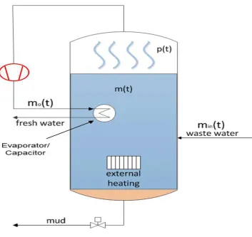
In Fig. 1a schematic representation of the considered system is shown. The system basically consists of the following three elements: a boiler, a compressor and an evaporator. In the boiler the waste water remains in the middle and lower part of it and in the upper part a vapor chamber is to be considered in order to host the water vapor which is generated by heating the waste water. At the beginning the mixture (waste water) is heated by a resistor system until the water vapor is present in the vapor chamber. At this time the heating is switched off and the compressor is switched on. The compressor should provide for a high pressure in the evaporator and in the meantime reduce the pressure in the vapor chamber through and a mass flow. This mass flow (m0(t)) after the condensed phase represents cleaned water in output of the evaporator and it is stilled. More in depth, in the evaporator, the vapor is condensed giving up heat to the waste water. To guarantee that new waste water can enter into the boiler from the upper part of it, the compressor provides a low pressure in the vapor chamber. In this sense, the compressor works as a controller in this process and its output is represented by the mass flowm0(t)with the constraint thatm0(t)>0. The compressor is equipped with an asynchronous motor which is controlled in frequency using an inverter piloted by a PWM signal which converts the output of the LMPC controller in frequency. In input to LMPC the pressure error is provided. More details of the control scheme will be given in the chapter devoted to the simulation. In any case, the dynamics of the asynchronous motor together with the inverter and all rest of the converters, considered all together, are much faster than the dynamics of the controlled process and in this analysis are not taken into account. Short description of the drain: At the beginning the pressure in the container equals the ambient pressure (circa 1.013 bar). By heating, the pressure increases slowly, as the water begins to evaporate. New water is added by a constant control with floats. The condensed water vapor from the "internal heat exchanger" is now free of foreign matter. For controller design purposes the dynamical model of the system must be considered. As already

(3)

Figure 1.Boiler system

explained, considering that the control process starts after the heating phase and more precisely when the water vapor becomes to be present in the boiler, the following equations can be considered:

dm(t)

dt =mi(t)−mo(t) dp(t)

dt = dm(t)

dt RgT

V ,

(1)

in whichmi(t)is a stepwise positive constant function. 38

39

Considering the Forward Euler discretisation with sampling timeTs, the following expression is

obtained:

m(k+1) =Ts(mi(k)−mo(k)) +m(k)

p(k+1) = (mi(k)−mo(k))R_VgT+p(k),

(2)

and thus 40

"

m(k+1) p(k+1)

#

| {z }

ˆ

z(k+1) =

"

Ts 0

0 1

#

| {z } Ak

"

m(k) p(k)

#

| {z }

ˆ

z(k) +

"

Ts TsRgT

V #

| {z } Bk

(mi(k)−m0(k))

| {z }

umpc(t)

(4)

4 of 10

3. Model predictive control

41

In the model approach just two samples are considered:

ˆ

z(k+1/k) =HkAkz(k/k) +HkBkumpc(k). (4)

If∆umpc(k) =umpc(k)−umpc(k−1), thenumpc(k) =∆umpc(k) +umpc(k−1)and 42

ˆ

yh(k+1) =HkAkzˆ(k/k) +HkBk(∆umpc(k) +umpc(k−1)). (5)

where matrixHkselects the second state variable and thusyh(t)represents the pressure.

ˆ

y(k+2) =HkA2kzˆ(k/k) +HkAkBk(∆umpc(k) +umpc(k−1)) +HkBk(∆umpc(k+1) +umpc(k)). (6)

It is straightforward to show that the following vectorial expression holds:

ˆ

Yh(k) =Gpx(k) +F1p∆Umpc(k) +F2pumpc(k−1), (7)

where

ˆ Yh(k) =

"

ˆ

yh(k+1)

ˆ

yh(k+2) #

, ∆Umpc(k) =

" _∆u mpc(k)

∆umpc(k+1), #

(8)

and matricesGp,F1pandF2pare given by:

F1p= "

HkBk 0

Hk(AkBk+Bk) HkBk #

, Gp=

"

HkAk

HkA2k #

, F2p=

"

HkBk

Hk(AkBk+Bk) #

. (9)

If the following performance criterion is assumed,

J= 1 2

N

∑

j=1

yd(k+j)−yˆ(k+j) T

Qp

yd(k+j))−yˆ(k+j)

+

N

∑

j=1

∆umpc(k+j) T

Rp(∆umpc(k+j)),

(10) whereyd(k+j),j=1, 2, . . . ,Nis the pressure reference profile andNthe prediction horizon, andQp

andRpare non-negative definite matrices. Index (16) can be written as

J= 1 2Yˆ

T

h(k)QpYˆh(k) +1

2∆U

T

mpc(k)Rp∆Umpc(k), (11)

then the solution minimizing performance index (11) may then be obtained by solving

∂J ∂∆Umpc

=0. (12)

A direct off-line computation may be obtained explicitly as

∆Umpc= (FT1pQpF1p+Rp)−1

FT₁_pQp Ydp(k)−Gpz(k)−F2pumpc(k−1)

, (13)

whereYdp(k)is the desired output column vector. For further details see [13].

43

(5)

44 4.AstabilitysufficientconstructiveconditioninGMPC

Theorem1. LetustakethediscreteSISOlinearsystemintoconsideration:

45

z(k+1) = Akz(k) +Bkumpc(k), (14)

y(k) = Hkz(k), (15)

obtained by a discretisation of a linear continuous system using a sampling time which equals Ts. umpc(k)

represents the first element of the vector of the optimal solution as calculated in [13] for the GMPC considering the following cost function:

J= 1 2

N

∑

j=1

yd(k+j)−yˆ(k+j) T

Qp

yd(k+j)−yˆ(k+j)

+

N

∑

j=1

∆umpc(k+j−1) T

·Rp∆umpc(k+j−1), (16)

where yd(k+j), j=1, 2, . . . ,N is the position reference trajectory and N is the prediction horizon, andQpand

Rpare non-negative definite matrices. Furthermore, the solution minimizing performance index (16) may be

obtained by solving:

∂J ∂∆Umpc

=0. (17)

It is known for instance from [13] that the optimal solution is: umpc(k) = (FT1pQpF1p+Rp)−1FT1pQp

Ydp(k)−Gpz(k)−F2pumpc(k−1)

, (18)

whereYdp(k)andYp(k)are the desired output column vector and the measured or observed output vector.

46

MatricesQpandRpare diagonal and positively defined. Under the technical hypotheses thatQp = I, and 47

HT_kH=Iare under the assumption

48

49

i) r₍_1,1₎>>T2

s, where r(1,1)represents the first diagonal element of matrixRp. 50

then∀r(1,1)such that:

r(1,1)>BkBTk

kAkk2

1− kAkk2, (19)

wherekAkk2represents the maximal eigenvalue of matrix

√

AT_A_and kAk−Bk

(FT₁_pQpF1p+Rp)−1FT1pQpGp

k2<kAk+Bk

k2, (20)

then the system (14) is asymptotically stable.

51

Proof 1. For sake of brevity just one prediction step is considered, then: F1p=

h

HkBk i

, (21)

F2p= h

HkBk i

, (22)

Gp= h

HkAk i

. (23)

Combining Eq. (14) with (18), this expression is got: z(k+1) =Akz(k) +Bk

(FT1pQpF1p+Rp)−1FT1pQp

Ydp(k)−Gpz(k)−F2pumpc(k−1)

(6)

6 of 10

which is equivalent to write:

z(k+1) =Ak−Bk

z(k)+ Bk

(FT₁_pQpF1p+Rp)−1FT1pQp

Ydp(k)

−Bk

F2p(k)

. (25)

If

r(1,1)>BkBTk

kAkk2

1− kAkk2, (26)

considering that scalar r(1,1)>0and scalarBkBT_k >0, then: 52

0<kAkk2+r−₍_1,11₎BkBTkkAkk2<1. (27) Recalling thatHT

kH=I 53

0<kAkk2+r₍−_1,11₎BkBTkHTkHkAkk2<1 (28) and thus

54

0<kAkk2+r−₍_1,11₎kBkBTkHTkHAkk2<1. (29) Being matrixF1pdefined as in (21) andG1pdefined in (23), it is known that matrixBk is proportional Ts, 55

then considering thatRp =r(1,1), choosing a suitable r(1,1)>>Tsand considering thatQp =I(technical 56

hypothesis), the following condition can be derived:

57

0<kAkk2+

Bk

2<1. (30)

Considering the norm properties and condition (20), then:

58

0<

Ak−Bk

(FT1pQpF1p+Rp)−1FT1pQpGp

2

<

Ak+Bk

2

<kAkk2+

Bk

₂<1. (31)

To conclude

59

0<kAkk − Bk

(FT1pQpF1p+Rp)−1FT1pQpGp

2<1. (32)

The constraint in (26) states a plausible condition on the controller. Stability represents the 60

necessary condition of the optimality of a controlled system. In order to interpret the result let us 61

observe a mechanical system including a mass-spring system in which it is known that the eigenvalue 62

can variate in the whole real and complex domain as a function of the mass which states the system 63

inertia. If massm →∞, then, because of the discretisation and according to the Landau notation, 64 λmax Ak −1

→ 0 withO λmax Ak −1

= O(_m1). In the meantimeO(BkBTk) = O(m12).

65

For a very slow system, according to (26),r(1,1)→0, parameterr(1,1)is present in the denominator

66

function of the optimal solution in (18) and in this case, small values ofr(1,1)are devoted to speed up

67

the system. If massm→0, then, because of the discretisation,O λmax Ak

=O1

m

, but in the 68

meantimeBkBTk →∞withO(BkBTk) =O(m12). For a very fast systemr(1,1)→∞, parameterr(1,1)is

69

(7)

devoted to slow down the system. So we can conclude that a highly inertial system needs relatively 70

small values ofr₍_1,1₎to be optimised and stabilised. If the inertia is small, then the system needs larger 71

values ofr(1,1)to be optimised and stabilised. In fact, very fast systems can have very high abrupt

72

changes in the input signals and in the cost function the input factor needs to be reduced to find an 73

optimality. 74

5. The saturation case

75

Proposition 1. Let us take the following discrete SISO linear system as before into consideration:

76

z(k+1) = Akz(k) +Bkumpc(k), (33)

y(k) = Hkz(k), (34)

and

|umpc(k)| ≤Umax ∀k, (35)

then (33) with the input saturation defined in (35) being asymptotically stable and its input avoiding the constraint if condition (26) holds together with the input limitation. The following condition summarizes the result:

r₍_1,1₎>max

(

BkBTkkYdp(k)k2 Umax

+

B_kF₁_pQ_pF₂_p

2 Umax

|umpc(k−2)|, BkBTk

kAkk2 1− kAkk2

)

. (36)

Proof 2. The demonstration is straightforward just considering that:

|umpc(k)|<|umpc(k)|<Umax ∀k

and thus it is enough that the following condition holds:

Bk

Ydp(k)

−Bk(FT1pQpF1p+Rp)−1F1pQpF2pumpc(k−1)

₂≤Umax.

(37) In fact, using similar considerations as before, the following expression is obtained:

Bkr

−1 11 FT1pQp

Ydp(k)

₂+|BkF1pQpF2p| ≤Umax, (38)

and thus, including also the stability condition, condition (36) follows here below again:

r(1,1)>max

(

BkBTkkYdp(k)k2 Umax

+

B_kF₁_pQpF2p ₂

Umax

|umpc(k−1)|, BkBTk

kAkk2 1− kAkk2

)

. (39)

It is possible to observe that for large values ofUmaxthe condition on the input barrier in the cost 77

function (16) with weightr(1,1)is not so restrictive, so larger inputs are allowed. For small values of

78

Umax the input barrier limits the values of the input and no large input values are allowed. 79

6. Simulation results

80

Concerning the simulation results, it is to be clarified that functionmi(t)is a stepwise constant

function withmi(t) =0.086 (kg/sec.) ormi(t) =0 and in the simulated casemi(t) =0.086 (kg/sec.)

is considered. As already explained, in the simulations two cases should be distinguished: weak anti-saturating action:

r(1,1)>

BkBTkkYdp(k)k2

(8)

8 of 10

and strong anti-saturating action:

r(1,1)>>

BkBTkkYdp(k)k2

Umax . (41)

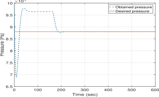
Fig. 2shows the controlled pressure which represents the main result. In case of anti-windup action being relatively weak, the anti-windup controller needs time to reestablish the control loop. As already explained, during the windup effect the feedback control is broken so the absence of the feedback control action can clarify the long permanence of the pressure at negative values. In particular, from Fig.3which represents the mass flow dm_dt(t) =min(t)−m0(t)(kg/sec) it is visible how this function is consequent with the relation:

dm(t) dt ≈

dp(t)

dt . (42)

Moreover, considering the following equation again:

dm(t)

dt =min(t)−m0(t), (43)

to activate the process a strong initial action through the mass flowm0(t)is required. Observing these 81

two figures it is possible too see that in the case of strong anti saturating action represented in Fig.5the 82

controlled system through the anti-windup scheme comes out from the saturation state very quickly 83

with a resulting faster dynamics. The resulting faster dynamics are obtained thanks to the stronger 84

anti-windup action which allows to reactivate the control loop very quickly. As already explained, 85

when the saturation occurs the control loop is open and no feedback control is present.

0 100 200 300 400 500 600

Time (sec.)

0.8 0.9 1 1.1 1.2 1.3 1.4 1.5 1.6

Pressure (Pa)

105

Obtained pressure Desired pressure

Figure 2.Desired and obtained pressure with weak anti-saturating action

86

7. Conclusion

87

One of the most important problems in the context of optimisation using LMPC is represented by 88

conservative conditions on the stability. This paper presents a sufficient and constructive condition for 89

the stability of an LGMPC calculating lower bounds of the element of matrixRwhich represent the 90

weights of the input in a typical given cost function. A physical interpretation of the result is given 91

on the light of some physical considerations. An illustrative example is provided in which a recover 92

water process is taken into consideration to test the proposed results through computer simulations. 93

(9)

0 100 200 300 400 500 600

Time (sec)

-5 -4 -3 -2 -1 0 1 2 3 4 5

Input mass flow m

i

(t)-m

o

(t) (kg/sec)

10-4

Figure 3.Mass flowm_dt(t) =min(t)−m0(t)(kg/sec) with weak anti-saturating action

0 100 200 300 400 500 600

Time (sec)

6.5 7 7.5 8 8.5 9 9.5 10

Pressure (Pa)

104

Obtained pressure Desired pressure

Figure 4.Desired and obtained pressure with strong anti-saturating action

References

94

1. Mercorelli, P. A switching Kalman Filter for sensorless control of a hybrid hydraulic piezo actuator using

95

MPC for camless internal combustion engines. Proceedings of the IEEE International Conference on

96

Control Applications, 2012, pp. 980–985.

97

2. Mercorelli, P. A switching model predictive control for overcoming a hysteresis effect in a hybrid actuator

98

for camless internal combustion engines. Proceedings of the IEEE PRECEDE 2011 - International Workshop

99

on Predictive Control of Electrical Drives and Power Electronics, 2011, pp. 10–16.

100

3. Qin, S.; Badgwell, T. A survey of industrial model predictive control technology. Control Engineering

101

Practice2003,11, 733–764.

102

4. Bolognani, S.; Peretti, L.; Zigliotto, M. Design and implementation of model predictive control for electrical

103

motor drives. IEEE Transactions on Industrial Electronics2009,56, 1925–1936.

104

5. Neelakantan, V.; Washington, G.; Bucknor, N. Model Predictive Control of a Two Stage Actuation System

105

using Piezoelectric Actuators for Controllable Industrial and Automotive Brakes and Clutches. J. Intel.

106

Mater. Syst. and Struct2008,19, 845–857.

(10)

10 of 10

0 100 200 300 400 500 600

Time (sec)

-6 -5 -4 -3 -2 -1 0 1 2

Input mass flow m

i

(t)-m

o

(t) (kg/sec)

10-3

Figure 5.Mass flowdm_dt(t) =min(t)−m0(t)(kg/sec) with strong anti-saturating action

6. Hu, Z.; Farson, D. Design of a waveform tracking system for a piezoelectric actuator. Proc. Inst. Mech.

108

Eng., J. Syst. Control Eng., 2008, Vol. 222, pp. 11–21.

109

7. Bemporad, A.; Morari, M.; Dua, V.; Pistikopoulos, E.N. The explicit linear quadratic regulator for

110

constrained systems.Automatica2002,38, 3–20.

111

8. Pedret, C.; Poncet, A.; Stadler, K.; Toller, A.; Glattfelder, A.; Bemporad, A.; Morari, M. Model-varying

112

predictive control of a nonlinear system. Internal report in Computer Science Dept. ETSE de la Universitat

113

Autònoma de Barcelona2000.

114

9. Liu, Y.C.; Lin, C.Y. Model Predictive Control with Integral Control and Constraint Handling for Mechatronic

115

Systems. Proc. of the 2010 International Conference on Modelling, Identification and Control; , 2010; pp.

116

424–429.

117

10. Mercorelli, P.; Goes, J.; Halbe, R. A Lyapunov based PI controller with an anti-windup scheme for a

118

purification process of potable water. 2014 International Conference on Control, Decision and Information

119

Technologies (CoDIT), 2014, pp. 578–583.

120

11. Mercorelli, P. An Optimal and Stabilising PI Controller with an Anti-windup Scheme for a Purification

121

Process of Potable Water. 16th IFAC Workshop on Control Applications of Optimization CAO’2015, 2015,

122

pp. 259–264.

123

12. Mercorelli, P. A sufficient asymptotic stability condition in generalised model predictive control to avoid

124

input saturation. Lecture Notes in Electrical Engineering2019,489, 251–257.

125

13. Sunan, H.; Kiong, T.; Heng, L.Applied Predictive Control; Springer-Verlag London: Printed in Great Britain,

126

2002.

127