Bandwidth Allocation under End-to-End Percentile Delay Bounds.

(1)

ABSTRACT

ANJUM, BUSHRA. Bandwidth Allocation under End-to-End Percentile Delay Bounds. (Under the direction of Harry Perros).

The main objective of this thesis is the estimation of the bandwidth that should be allocated on each link along the path of a flow of IP packets, so that the end-to-end delay D is bounded statistically. That is, D is less than or equal to a given value T with a probability γ. The path through an IP network is depicted by a tandem queueing network of infinite capacity queues, where each queue represents the output port of a router.

We first obtain some results on adding percentiles, and then we propose two different algorithms for calculating end-to-end percentiles, which is then used in a simple search algorithm to obtain the required bandwidth. The first algorithm is based on probabilistic assumptions regarding the arrival process of the packet flow and service times at each node in the tandem queueing network. The second algorithm is based on traces, such as video traces, that consist of a sequence of tuplets, each describing the time of arrival of a packet and its packet length.

In the first algorithm, we assume that the arrival process to the first queue of the queueing network is bursty and correlated and the service times are exponentially distributed. Initially, we assumed an MMPP (Markov-modulated Poisson process) arrival process, and then we extended the algorithm to a MAP2 (two-stage Markov arrival process) arrival process. A MAP can represent a variety of processes that includes, as special cases, the Poisson process, the phase-type renewal processes, the MMPP and superposition of these. No background arrivals were considered at each node, the implication being that the output port scheduler is assumed to be per flow. The proposed algorithm is based on an interpolation between an upper and lower bound obtained by analyzing only the first queue. It is a relatively simple algorithm despite the complexity of the problem, and as shown through extensive comparisons with simulation data that it has a very low relative error. The average error is 1.25% for MMPP and 4.5% for MAP2.

(2)

150 to 200 msec in order to guarantee good QoE. Interestingly enough, little is known about how much bandwidth should be allocated to an interactive video so that a given percentile of the end-to-end delay is satisfied. Using the above algorithm, we obtained the end-to-end percentile for video traffic, by approximating a video trace with a MAP2. Subsequently, the required bandwidth so that a given end-to-end percentile is satisfied is obtained using a simple search algorithm. Three different types of video traces were used, namely, Cisco’s Telepresence, IPTV and WebEx. The approximation of video trace by a MAP2 coupled with the above algorithm gives results with a low relative error, the average relative error is around 6%.

(3)

Bandwidth Allocation under End-to-End Percentile Delay Bounds

by Bushra Anjum

A dissertation submitted to the Graduate Faculty of North Carolina State University

in partial fulfillment of the requirements for the degree of

Doctor of Philosophy

Computer Science

Raleigh, North Carolina 2012

APPROVED BY:

Dr. William Stewart Dr. David Thuente

Dr. Harry Perros

Chair of Advisory Committee

(4)

ii

DEDICATION

To Mom!

(5)

iii

BIOGRAPHY

(6)

iv

ACKNOWLEDGEMENTS

(7)

v

LIST OF TABLES

Table 1.1 Scheduling Policies ... 9

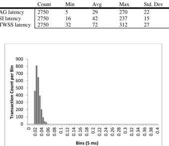
Table 2.1 Population statistics in ms... 46

Table 2.2 A comparison of percentiles ... 48

Table 3.1 Squared-coeffficient of variation of the departure process. ... 65

Table 3.2 Relative Errors ... 69

Table 5.1 Statistics of Multiplexed Telepresence Traces ... 101

Table 5.2 Statistics of Resultant Trace as multiple WebEx traces get multiplexed together 105 Table 5.3 Statistics of Resultant Trace as multiple IPTV traces get multiplexed together .. 108

(12)

x

LIST OF FIGURES

Figure 2.1 Composition of n components ... 22

Figure 2.2 A sequence of exponential distribution ... 23

Figure 2.3 Erlang-n versus sum of n exponentials ... 24

Figure 2.7 95th percentile of Erlang-n and using weight function ... 28

Figure 2.8 99th percentile of Erlang-n and using weight function ... 29

Figure 2.9 Hypoexponential-n versus sum of n exponentials ... 31

Figure 2.10 Hypoexponential-n versus sum of n exponentials ... 31

Figure 2.11 95th percentile of hypoexponential-2 and equation 12 ... 33

Figure 2.16 Coxian-n distribution ... 37

Figure 2.17 Coxian-2 distribution ... 37

Figure 2.18 A series of Coxian 2 distributions ... 38

Figure 2.19 95th percentile of phase type and equation 14 ... 40

Figure 2.20 95th percentile of phase type and equation 14 ... 40

Figure 2.21 7 component network model ... 42

(13)

xi

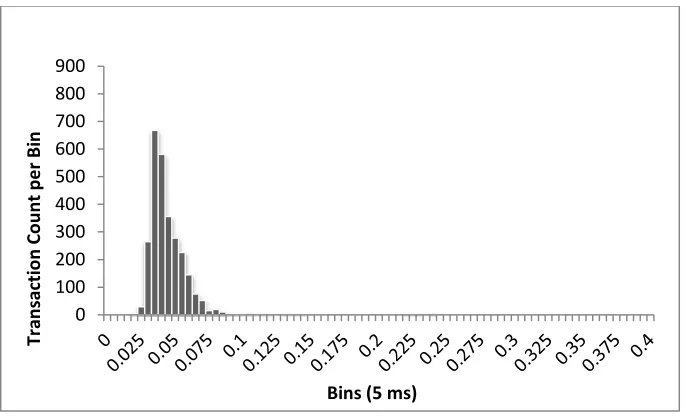
Figure 2.23 AG latency data ... 46

Figure 2.24 SI latency data ... 47

Figure 2.25 TWSS latency data ... 47

Figure 2.26 The network under study ... 49

Figure 2.27 The minimum spanning tree using the average delay ... 49

Figure 2.28 The minimum spanning tree using the percentile delay ... 50

Figure 3.1 The tandem queueing network under study... 55

Figure 3.2 The phase type distribution of the end-to-end delay ... 58

Figure 3.3 The CDF of D, D1, and D ... 60

Figure 3.4 The upper and lower bounds of the bandwidth ... 62

Figure 3.5 Bandwidth results for a tandem network with 10 queues ... 64

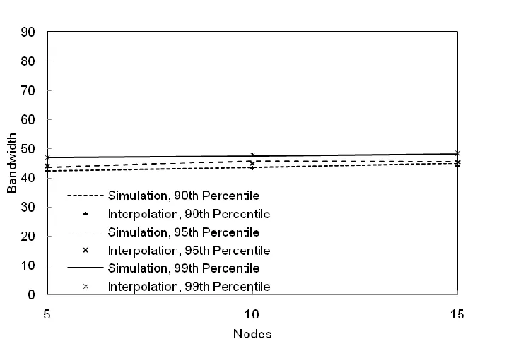
Figure 3.6 Interpolation function vs simulation for various delay percentiles ... 66

Figure 3.7 Interpolation function vs simulation for various values of the delay T ... 67

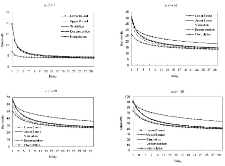
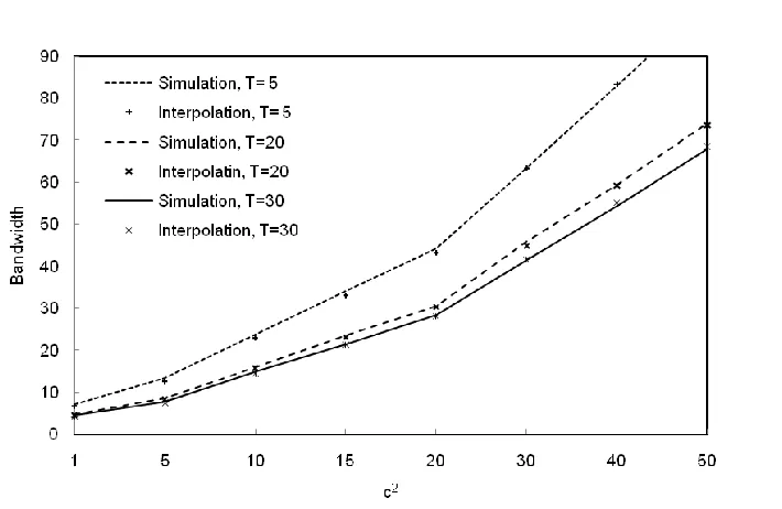
Figure 3.8 Interpolation function vs simulation for various c2 values ... 67

Figure 3.9 Interpolation function vs simulation for various ρ values ... 68

Figure 3.10 Bandwidth results for a tandem network with 10 queues for a single IPP. ... 70

Figure 4.1 The tandem queueing network under study... 76

Figure 4.2 The upper and lower delay bounds ... 81

Figure 4.3 95th Percentile Delay results for a Tandem Network with 10 queues ... 84

Figure 4.4 Telepresence Trace. Packet Length Distribution (left), Arrival Bit Rate (right) ... 86

Figure 4.5 Telepresence Trace. The 95th Percentile of the T vs. Utilization (left), Bandwidth Required vs. TD(right) ... 87

(14)

xii

Figure 4.7 IPTV Trace. The 95th Percentile of the T vs. Utilization (left), Bandwidth

Required vs. TD(right) ... 89 Figure 4.8 WebEx Trace. Packet Length Distribution (left), Arrival Bit Rate (right) ... 89 Figure 4.9 WebEx Trace. The 95th Percentile of the T vs. Utilization (left), Bandwidth

Required vs. TD(right) ... 90 Figure 5.1 Tandem Queueing Network under study ... 96 Figure 5.2 Infinite Looping of Trace to create Background Traffic ... 101 Figure 5.3 Burstiness (left) and Autocorrelation (right) of combined Telepresence streams102 Figure 5.4 Bandwidth Requirement for Fixed 95th Percentile Delay of 30msec (left).

Difference between No Statistical Gain and Required BW (right) ... 103 Figure 5.5 Bandwidth Requirement for Fixed 95th Percentile Delay of 50msec (left).

Difference between No Statistical Gain and Required BW (right) ... 104 Figure 5.6 Bandwidth Requirement for Fixed 95th Percentile Delay of 70msec (left).

Difference between No Statistical Gain and Required BW (right) ... 104 Figure 5.7 Burstiness (left) and Autocorrelation (right) of combined WebEx streams ... 106 Figure 5.8 Bandwidth Requirement for Fixed 95th Percentile Delay of 30msec (left).

Difference between No statistical Gain and Required BW (right) ... 107 Figure 5.9 Bandwidth Requirement for Fixed 95th Percentile Delay of 50msec (left).

Difference between No statistical Gain and Required BW (right) ... 107 Figure 5.10 Bandwidth Requirement for Fixed 95th Percentile Delay of 70msec (left). Difference between No statistical Gain and Required BW (right) ... 108 Figure 5.11 Burstiness (left) and Autocorrelation (right) of combined IPTV streams ... 109 Figure 5.12 Bandwidth Requirement for Fixed 95th Percentile Delay of 1 sec (left).

Difference between No statistical Gain and Required BW (right) ... 110 Figure 5.13 Bandwidth Requirement for Fixed 95th Percentile Delay of 2 sec (left).

(15)

xiii

Figure 5.14 Bandwidth Requirement for Fixed 95th Percentile Delay of 3 sec (left).

Difference between No statistical Gain and Required BW (right) ... 111

Figure 5.15 Markov Chain of an IPP ... 112

Figure 5.16 Markov Chain of an (n+1) state MMPP representing n aggregate IPPs ... 113

Figure 5.17 Bandwidth Requirement for Fixed 95th Percentile Delay of 50 msec ... 113

Figure 5.18 Difference between No statistical Gain and Required BW ... 114

Figure 5.19 Pictorial Representation of big-theta ϴ ... 116

Figure 5.20 The 95th percentile delay (left) and jitter (right) calculated end-to-end, and for nodes 1, 2 and 3 when the background load on all three nodes increases proportionately .. 120

Figure 5.21 The 95th percentile delay (left) and jitter (right) calculated end-to-end, and for nodes 1, 2 and 3. Constant background traffic for nodes 1 and 3 while the background load on node 2 increases. ... 121

Figure 5.22 The 95th percentile delay (left), and jitter (right) calculated end-to-end, and for nodes 1, 2 and 3. Constant background traffic for nodes 1 and 2 while the background load on node 3 increases. ... 121

Figure 5.23 The 95th percentile delay (left), and jitter (right) calculated end-to-end, and for nodes 1, 2 and 3 when the background load on all three nodes increases proportionately .. 122

Figure 5.24 The 95th percentile delay (left), and jitter (right) calculated end-to-end, and for nodes 1, 2 and 3. Constant background traffic for nodes 1 and 3 while the background load on node 2 increases. ... 123

Figure 5.25 The 95th percentile delay (left) and jitter (right) calculated end-to-end, and for nodes 1, 2 and 3. Constant background traffic for nodes 1 and 2 while the background load on node 3 increases. ... 123

Figure 5.26 Bandwidth and Jitter values for a 95th Percentile Delay of 50msec ... 124

Figure 5.27 Bandwidth and Percentile Delay values for Jitter of 10msec ... 125

(16)

xiv

Figure 5.29 Required bandwidth for dual bounds ... 127

Figure 5.30 Bandwidth and Jitter values for 95 Percentile Delay of 50msec ... 128

Figure 5.31 Bandwidth and Percentile Delay values for Average Jitter of 10msec ... 128

Figure 5.34 Bandwidth and Jitter values for 95 Percentile Delay of 50msec ... 130

Figure 5.35 Bandwidth and Percentile Delay values for Average Jitter of 10msec ... 131

(17)

1

Chapter 1

1 Introduction

1.1 End-to-End Quality of Service

Quality of Service (QoS) refers to the capability of a network to provide service differentiation for certain types of traffic. The primary goal of QoS is to provide specific traffic guarantees: controlled delay and jitter, bandwidth, and packet loss characteristics. Also it is important to make sure that providing priority to one type of traffic does not make the QoS of other traffic fail. Fundamentally, QoS can provide for better service to certain traffic by guaranteeing network resources that satisfy the user’s demand. A key feature is that a network can provide different QoS levels to different services and each service has its own set of QoS requirements. For example, for an acceptable voice conversation over the Internet, it is recommended to have a one-way latency below 150 ms, a delay variation of about 30 ms, and a packet loss ratio below 1 percent.

(18)

2

review various schemes and concepts that have been standardized by Internet Engineering Task Force (IETF) so that to provide QoS in IP networks.

1.2 IP Network QoS Architectures

The IP-based Internet has not been designed to support QoS guarantees. This stems from the fact that the original Internet applications (e.g., email and FTP) are data oriented and they had little or no need for stringent guarantees. However, in the new era marked by the growing interest in providing voice and video services over IP networks, this situation is rapidly changing. This trend is paralleled by a phenomenal growth of the World Wide Web, with voice and video being further integrated into the design of Web pages. Given these recent trends, the IETF has been exploring various options for supporting multimedia traffic over IP.

1.2.1 Real Time Protocol (RTP)

RTP is the first step of supporting voice and video over Internet. RTP runs on top of UDP and interfaces it with the audio or video application. It is a session layer protocol and is transparent to network routers. Resultantly, it cannot be used to support network level QoS guarantees, still, it provides several functions useful for real time communications, including sequence numbering, timestamping, payload type identification etc. There are various ways of assigning RTP streams to media sources. Taking the example of teleconferencing, one may assign an RTP stream to each voice or video source in each direction. Alternatively, one RTP stream per voice and video bundle (as in case of MPEG) may also be assigned in each direction.

(19)

3

control protocol (RTCP) to convey various types of information, including the number of transmitted packets and the number of lost packets. This information can be used by the sender to adjust the compression parameters and reduce the bit rate if necessary. In other words, RTP is best suited for adaptive video applications.

1.2.2 Integrated Services (IntServ)

Integrated Services Working Group of the IETF has developed a framework for Integrated Services (IntServ) that can support some form of QoS guarantees over the Internet in the 1990s. IntServ is a per-flow-based QoS framework with dynamic resource reservation. A specific flow, defined by the vector ‘IP source address, IP destination address, TCP/UDP source port, TCP/UDP destination port’, is recognized in the network and may deserve a specific treatment. Integrated services are based on an ATM-like paradigm, where each source–destination flow is distinguished. This implies the use of resource reservation, packet scheduling and buffer management, exactly as in ATM technology. It requires that routers through which a path traverses keep information about the status of the flow and that the status is periodically refreshed. IntServ uses the resource reservation protocol (RSVP) [1] to signal requests. The IntServ framework consists of two service offerings: Guaranteed Service [2] and Controlled Load Service [3]. The former guarantees a reliable upper bound on the metric ‘end-to-end packet delay’ based on worst-case assumption. The bound guarantee implies the use of control mechanisms as access control and traffic policing. By guaranteeing a certain bandwidth, the network guarantees the associated maximum packet delay (packet loss is guaranteed to be zero). The latter is aimed at providing a service similar to the level that a non-congested router would provide; it does not provide any upper bound but still requires packet scheduling and buffer management on per-flow basis.

(20)

4

reserves the correct queueing preferences for the flow, such that the appropriate amount of bandwidth is allocated to the flow by the queueing tool.[4]. The second component, IntServ admission control, decides when a reservation request should be rejected. It is important because if all requests were accepted, eventually too much traffic would be introduced into the network, and none of the flows would get their requested service.

IntServ does not scale up well since the state of each path in each router is soft and as a result it needs to be continuously refreshed. Its signaling protocol RSVP, however, was reused successfully in MPLS.

1.2.3 Differentiated Services (Diffserv)

DiffServ [5] has been proposed by IETF in late 1990s with scalability as the main goal. In contrast to the IntServ model, Diffserv does not distinguish each traffic flow and resultantly it does not require a reservation protocol. It rather relies on the agreements between ISPs and clients to provide QoS guarantees. Classification of packets is performed based on the Differentiated Services (DS) field, which is part of the original ToS byte, in the header of an IP packet. Based on the field, the packets are classified into service classe, which are also referred as per hop behavior (PHB), when they enter the network. There are four main PHBs defined: assured forwarding (AF), expedited forwarding (EF), class selector (CS) and best effort (BE).

1.2.3.1Assured Forwarding

The AF classes of PHB were designed to support data applications with assured bandwidth requirements. That is, packets will be forwarded with a high probability as long as the class rate submitted by the user does not exceed predefined contracted rate.

(21)

5

Typically, routers drop packets when a queue, in which the router needs to place the packet, is full. This action is called tail drop. Congestion Avoidance starts discarding packets before tail drop is required, hoping that the source will be notified early and eventually, fewer packets will be dropped,

1.2.3.2Expedited Forwarding

The EF PHB is used to support applications that require low delay, low jitter, low packet loss, and assured bandwidth, such as VoIP.

The EF class suggests two QoS actions be performed to achieve the PHB. First, queueing must be used to minimize the time that EF packets spend in a queue. To reduce delay, the queueing tool should always service packets in this queue next. Also, anything that reduces delay reduces jitter. In addition to that, by always servicing the EF queue first, the scheduling discipline greatly reduces the queue length, which in turn greatly reduces the chance of tail drop due to the queue being full. Therefore, EF's goal of reducing delay, jitter, and loss can be achieved with a queueing method/scheduling discipline such as Priority Queueing. The second component of the EF PHB is policing. Policing implies that if the input load of EF packets exceeds a configured rate, the excess packets are discarded. Thus, EF protects other traffic types by capping the amount of bandwidth for the class.

1.2.3.3Class Selector

CS PHB is used for backward compatibility with IP precedence ToS field. It uses the "bigger-is-better" logic, i.e., the bigger the value in DS field, the better the QoS treatment.

1.2.3.4Best Effort

The default BE PHB has no committed resources and yet it cannot be starved by other PHBs. This is usually supported by allocating some nominal bandwidth to the BE flows.

(22)

6

dropping them increases when there is congestion in the core). A good example of a policer is the single rate three color marker scheme. The green, yellow and red actions have to do with dropping and marking of a packet. Typical action is as follows. Green action means that the packet is conformant and it should be let into the network. Yellow action means that the packet is not conformant, but it can be marked and let into the network. Finally, red action means that the packet is not conformant and it will be dropped. [6] Each node within the network then applies different queueing and dropping policies on every packet based on the marking that packet carries.

DiffServ is aimed at overcoming the scalability problem mentioned for the integrated services and does not require per-flow state and signaling. In practice, traffic is divided into classes that deserve a common service in the network. The advantage stands in the aggregation of many flows into a single traffic class, whose packets are forwarded in the same way in a router. This permits DiffServ to scale up to large size networks. However, the drawback is that no service per-flow can be guaranteed. So, while IntServ has inherent scalability problems, DiffServ does not provide explicit means for the application to negotiate a service level with the network. Also, unlike RSVP/IntServ, DiffServ needs to be provisioned. Setting up the various classes throughout the network requires knowledge of the applications and traffic statistics for aggregates of traffic on the network. This process of application discovery and profiling can be time-consuming. Still, DiffServ is widely used in the Internet, and it predates MPLS. Also some models using IntServ at the edge and DiffServ at the core of the network have been proposed [7]

1.2.4 Traffic Engineering

(23)

7

Engineering (TE) and MPLS come into service. True QoS, with maximum network utilization, will arrive with the combination of traditional QoS and routing.

Traffic Engineering refers to the process of selecting the paths chosen by data traffic in order to facilitate efficient and reliable network operations while simultaneously optimizing network resource utilization and traffic performance. The goal of TE is to compute path from one given node to another such that the path does not violate any constraints (bandwidth/administrative requirements) and is optimal with respect to some scalar metric. Once the path is computed, TE is responsible for establishing and maintaining forwarding state along such a path.

The lack of per-flow mechanisms in the DiffServ approach can be bypassed by proper traffic engineering techniques that assign a proper dimension to the bandwidth pipe assigned to each traffic class. Aref Meddeb, ISIT Com, in [8] showed that DiffServ offers bandwidth savings, relatively simple deployment, and tight SLA capabilities, especially when combined with TE. However, the benefit of DiffServ-aware TE does not seem to justify its complexity as surveyed by X. Xio in [9]. Furthermore, A. Mohammad et al [10] states that “DiffServ cannot commit to any specific value of delay or jitter without the help of other protocols or mechanisms such as bandwidth brokers or MPLS.”

1.2.5 Multiprotocol label switching (MPLS)

(24)

8

MPLS is a technology convergence between ATM and IP [11] [12]. MPLS sets up paths in a network along which packets that carry appropriate labels can be forwarded very efficiently (i.e. the forwarding engine does not use at the IP address, rather it uses the label to forward the packet). Not only does this allow packets to be forwarded more quickly, it also allows paths to be set up in a variety of ways: the path could represent the normal destination-based routing path, it could represent a policy-based explicit route, or it could represent a reservation-based flow path. Ingress routers classify incoming packets and wrap them in an MPLS header that carries the appropriate label for forwarding by the interior routers. In the MPLS model, the labels are distributed by the RSVP-TE, which is an extension of RSVP, and which sets up effectively a label switched path (LSP) along the label switched routers (LSR). RSVE-TE can be used to set up LSPs using the forwarding table (e.g. OSPF) or explicit routes based on maximizing one or more QoS parameters as well as taking into account policy-based rules. It is important to note that this label state can be per flow (as it was with IntServ) but usually represents some aggregate (e.g. between some source–destination pair). Therefore, the state produced by MPLS is manageable and scalable [13]

1.2.6 MPLS Overlay Networks

Although MPLS label switching provides the underlying technologies in forwarding packets through MPLS networks, it does not provide all the components for Traffic Engineering support such as traffic engineering policy. The existing Interior Gateway Protocols (IGP) are not adequate for traffic engineering. Routing decisions are mostly based on shortest path algorithms that generally use additive metric and do not take into account bandwidth availability or traffic characteristics.

(25)

9

These capabilities allow easy movement of traffic from an over subscribed link to an underused one.MPLS is the overlay model used by Traffic Engineering

1.2.7 Queue Management and Scheduling Policies

In the interior routers, differentiated packets have to be handled differently. To do so, the router may employ multiple queues, along with some class-based queueing (CBQ) service discipline or simple priority queueing. Generally, delay-sensitive traffic will be serviced sooner, and loss-sensitive traffic will be given larger buffers. The loss behaviour can also be controlled using various forms of random early detection (RED). These disciplines using probabilistic methods to start dropping packets when certain queue thresholds are crossed, in order to increase the probability that higher quality packets can be buffered at the expense of more dispensable packets. Some of the widely used scheduling policies are described in the table below

Table 1.1 Scheduling Policies

Scheduling Policy Queue Service Algorithm

Priority Queueing (PQ)

Strict service; always serves higher-priority queue over lower queue

Custom Queueing (CQ)

Serves a configured number of bytes per queue, per round-robin pass through the queues. Result: Rough percentage of the bandwidth given to each queue under load Weighted Fair

Queueing (WFQ)

Each flow uses a different queue. Queues with lower volume and higher IP precedence get more service; high volume, low

precedence flows get less service. Class-Based

Weighted Fair Queueing (CBWFQ)

Results in set percentage bandwidth for each queue under load.

Low Latency Queueing (LLQ)

LLQ is a variant of CBWFQ, which makes some queues "priority" queues, always getting served next if a packet is waiting in that queue. It also polices traffic.

Modified Deficit Round-Robin (MDRR)

(26)

10

1.3 End-to-end Bandwidth Guarantees

As discussed in the previous section, MPLS is able to provide end-to-end bandwidth guarantee whereas DiffServ is generally unable to do so. This is mainly because though an ISP can have a general idea of the traffic entering his network, he does not have any control on the path followed by the traffic or the domains it pass through. End-to-end quality of service usually requires a method of coordinating resource allocation between one autonomous system and another. IntServ can also provide bandwidth guarantees but it is not used much due to its scalability issues.

From this point onwards, we will consider an MPLS network and we will focus on the problem of calculating bandwidth for an LSP to ensure a quality experience for the user when certain characteristics about the arrival traffic are known. It is interesting to note that the term “quality experience” has different meanings for different applications. For example for real time voice, the primary concern will be to minimize end-to-end delay but it is resilient to some packet loss. Whereas a data centric application like FTP requires zero packet loss but can endure network delays. There is a spectrum of applications with different quality requirements and expectations from the network. Generally, there are two ways of doing bandwidth allocation; one is to guarantee packet loss and the other to bound end-to-end delay and jitter. Below we give a brief survey of techniques for guaranteeing packet loss. The subject matter of this thesis is bandwidth allocation under end-to-end delay guarantees and a detailed review of the relevant literature is given in the following section 1.3.2.

1.3.1 Bandwidth allocation based on Packet Loss

(27)

11

bandwidth allocation to the aggregate traffic results in a reduction in the per stream allocated bandwidth, where the reduction is proportional to the burstiness of the multiplexed sources.

Several queueing theoretic papers have analyzed the loss probability in finite buffers or the queueing tail probability in infinite buffers. For instance, Kim and Shroff model the input traffic as a general Gaussian process and derive an approximate expression for the loss probability in a finite buffer system [15].

An early experimental study by Villamizar and Song recommended that the buffer size should be equal to the bandwidthdelay product (BDP) of that link [16]. The “delay” here refers to the RTT of a single and persistent TCP flow that attempts to saturate that link, while the “bandwidth” term refers to the capacity C of the link. That rule requires the bottleneck link to have enough buffer space so that the link can stay fully utilized while the TCP flow recovers from a loss-induced window reduction.

The BDP rule results in a very large buffer requirement for high-capacity long-distance links. At the same time, such links are rarely saturated by a single TCP flow. Appenzeller et al. concluded that the buffer requirement at a link decreases with the square root of the number N of “large” TCP flows that go through that link [17]. According to their analysis, the buffer requirement to achieve almost full utilization is B=(CT)/ , where T is the average RTT of the N (persistent) competing connections. The key insight behind this model is that when the number of competing flows is sufficiently large, which is usually the case in core links, the N flows can be considered independent and nonsynchronized, and so the standard deviation of the aggregate offered load (and of the queue occupancy) decreases with . An important point about this model is that it aims to keep the utilization close to 100% without considering the resulting loss rate.

(28)

12

link fully utilized by a set of N heterogeneous TCP flows while keeping the loss rate and queueing delay bounded.

Recently, the ACM Computer Communications Review (CCR) has hosted a debate on buffer sizing through a sequence of letters [19], [20], [21], [22]. On one side, Enachescu et al in [20] and Raina et al in [21] have proposed significant reduction in the buffer requirement based in results from earlier studies [17]. They argue that 100% link utilization can be attained with much smaller buffers, while large buffers cause increased delay, induce synchronization, and are not feasible in all-optical routers. On the other side of the debate, Dhamdhere and Dovrolis in [19] and Vu-Brugier et al in [22] highlight the adverse impact of small buffer size in terms of high loss rate and low per-flow throughput. Dhamdhere and Dovrolis argued that the recent proposals for much smaller buffer sizes can cause significant losses and performance degradation at the application layer [19]. Similar concerns are raised by Vu-Brugier et al. in [22]. That letter also reports measurements from operational links in which the buffer size was significantly reduced.

Lakshmikantha et al. [23] have showed that depending on the ratio between the “edge” and “core” link capacities, the buffer requirement can change from O(1) (just few packets) to O(CT) (in the order of the BDP).

1.3.2 Bandwidth allocation based on end-to-end delay

A well known approach of allocating bandwidth so as to guarantee end-to-end delay is called equivalent bandwidth, proposed originally for ATM networks, see Perros [6]. In addition, a survey of various call admission algorithms can be found in Wright [24].

(29)

13

interested in finding out the worst case end-to-end delay of the system. The end-to-end traffic is characterized using Virtual Links (VL) where a VL is defined as a logical unidirectional connection from one source port to one or more destination ports. Hence, VL is a path with multicast characteristics. The first approach used to evaluate the upper bound end-to-end delay is that of network calculus. Given an elementary entity that offers service curve β to an input flow constrained by an arrival curve α, the calculus brings the arrival curve α* of the output flow: α*=αØβ where αØβ defined by: . Using a Network Calculus tool to propagate these results on the complete network, the approach analytically derives sure upper bounds on delays. However, the bounds are extremely pessimistic as observed when crossed checked by the experimental upper bounds obtained by simulation of a set of scenarios. The ratio of the end-to-end delay obtained by simulation and the one calculated with the network calculus is mostly between 5% and 40% with the ratio 70% achieved only when all VL paths have a length 1. However, simulation model may miss rare events hence undermining the worst case delay and so a more comprehensive approach of modeling the network as timed automata with model checking may be used. It gives an exact worst case end-to-end delay by exploring all the possible states of the system. However the number of states is directly dependent on the size of the output queues per switch and the external arrivals and may lead to combinatorial explosion.

(30)

14

K times to get the end-to-end delay value on which a γ-percentile may be constructed. Experimental evidence shows that in access networks (low bit rates) the improvement over the upper bound, due to the later method, can be up to 45% and in the order of tens of milliseconds, whereas in core networks (high bit rates) the upper bound is reasonably accurate in predicting the end-to-end delay.

Vleeschauwer et al [27] have described four different approximations to compute the γ-percentile of the total queueing delay in a heterogeneous network where each node can be represented by an M/G/1 queue. The queues are assumed to be independent, but not necessarily identical. The simplest approximation is based on the assumption that the distribution of the total queueing delay, consisting of N statistically independent queueing delays, shapes towards a Gaussian distribution. Hence the percentiles can be calculated as: µ + erfc-1(P) where erfc is the complimentary error function of the Gaussian distribution. A heuristic formula is subsequently developed along the same lines but this time the weighing factor instead of being erfc is chosen such that , the formula would be exact if the individual delays were exponentially distributed. The third approach is based upon the dominant pole associated with each M/G/1 node. If the moment generating function of the delay in one node can be written as: Dn(s)=Hn(s)/(s-pn), where (s-pn) is the dominant pole, the end-to-end distribution is a weighted sum of the CDFs of Erlang variables. Experimental evidence shows that the second and third approach outperforms Gaussian approximation in all cases, the main reason being that a very large number of nodes (order of a few hundred) is required to make the resultant CDF a Gaussian distribution. Whereas the errors for the two methods are smaller than 1% as soon as the load on at least one of the nodes is high enough (0.7 for second method and 0.5 for the third method). The last method discussed involves the numerical inversion of the Laplace transforms following Abate and Whitt [28]. This method is the most complicated one but it works very well but not for very high percentiles because of the discretization and truncation errors which are inherent in the method.

(31)

15

algorithms. The authors define Guaranteed Rate algorithms (GR) as a class of schedulers that can guarantee a deadline by which a packet of an accepted flow will be transmitted, e.g., virtual clock, self clocked fair queueing, generalized processor sharing. Using the arrival time of the packet, transmission deadline calculated by the first scheduler, packet length and the flow’s associated rate per node, a mathematical upper bound is constructed that is shown to work well with the sources conforming to Leaky Bucket and Exponentially Bounded Burstiness.

Lehoczky and Yeung [30] work on a new queueing theory methodology called real-time queueing theory, that allows one to keep track of the deadlines associated with each of the tasks/packets in the system. An important performance metric in this theory is the packet lateness probability i.e., the fraction of packets which miss their deadline. The theory can be applied only when the traffic intensity on the server approaches 1. In this case, under very general circumstances (general i.i.d interarrival time and service time distributions), the occupancy of the queueing network can be treated as a reflected Brownian network process with drift whose equilibrium probability distribution is of product form if the first two moments of the interarrival time and service time distributions satisfy certain conditions. Considering a simple two stage distributed network and using the product form solution, the authors computed a closed form expression of the PDF of the end-to-end delay further from which the proportion of late packets of each session is determined. The authors provide closed form expressions for the proportion of late packets for two scheduling disciplines EDF and FIFO and for constant and uniform distributed deadlines. Simulations illustrate good accuracy of the closed form expressions.

(32)

16

packets is derived on the basis of single packet results. Second major contribution is the derivation of explicit expressions for expected waiting time in the queue for each of the priority classes. The paper also formulates the embedded Markov chain of the G/M/1 node by considering all possible states and derives the corresponding transition probabilities.

An exact numerical expression of the end-to-end delayin a tandem queueing network can also be obtained by calculating its Laplace transform and then inverting it numerically to obtain delay percentiles. This approach was used by Xiong and Perros, [32] within the context of resource optimization of web services using a tandem queueing network with Poisson arrivals and exponentially distributed service times.

Yeung and Lehoczky [33] used a Brownian process to study a two-stage queueing network with customers having deadlines (constant and uniformly distributed) and calculated bounds for two different scheduling disciplines, early-deadline first and FIFO. Fractional Brownian Motion (FBM) was used by Lelarge et al [34] to show that the end-to-end delay of a tagged flow in a tandem queueing network, and more generally in a tree network, is completely dominated by the queue with the maximal Hurst parameter.

1.4 Summary of the Thesis

The rest of the thesis is organized as follows. In Chapter 2, we define percentiles and discuss their statistical significance in various networking situations. We then present an exact analytic expression for adding percentiles of random variables whose PDF is a mixture of exponentials. Specifically we have considered exponential, Erlang, hypoexponential, hyperexponential, and Coxian-2 distributions. We also discuss the applicability of percentile calculations to routing protocols, presenting Dijstra’s algorithm as an example.

(33)

17

less than or equal to a given target delay value T with a probability γ, i.e., P(D≤T) = γ. We assume that the arrival of packets follow an MMPP2 process, because it is capable of capturing burstiness and autocorrelation characteristics commonly present in network traffic while satisfying a reduced complexity. We first construct an upper and a lower bound on a given percentile of D, from which we obtain bounds of the bandwidth such that P(D≤T) = γ, for given T and γ. These two bounds are then combined using an interpolation function to obtain an accurate estimate of the bandwidth. The main contribution of the scheme is that the upper and lower bounds are constructed by analyzing only the first queue of the tandem queueing network.

In Chapter 4, we extend the approach described in Chapter 3 to the case where the arrival process is a two-state Markov arrival processes (MAP). A MAP can represent a variety of processes that includes, as special cases, the Poisson process, the phase-type renewal processes, the MMPP and superposition of these. Later in the chapter, we also used a MAP2 to successfully approximate the packet arrival process of various video streams, such as Cisco’s Telepresence, IPTV and WebEx.

(34)

18

(35)

19

Chapter 2

2 Percentile Arithmetic

2.1 Introduction

Let us consider a performance metric such as the response time of a router or a web service or a software process. Typically, we use the average of this metric as an indicator of its performance. For instance, we will say that the average time it takes for a specific web service is 2 ms. However, we all know that averages can be misleading as they do not represent the range of values of the response time under study. On the other hand, a percentile of the metric provides a better understanding than the mean value, since it bounds statistically the behavior of a system. The c percentile, such as 95th percentile, of a variable X is a value below which X lies c% of the time.

(36)

20

Response time in a web service: The execution of a web-based service may involve several sites, each carrying out part of the service flow. Given that each site can guarantee the 95th percentile of its own response time, the question is what is the 95th percentile of the total end-to-end time. This end-to-end percentile can then be used in the negotiation of the contract with the user.

Testing a large suite of software: Let us consider a suite of software components that provide a service. Such a suite can be the set of software designed to provide IMS services. Testing for bottlenecks is standard routine before the software is released. However, due to the complexity of IMS, it is impossible to have all the components present in a lab. In view of this, the components that are not available for testing are often represented by idealized simulations which are generally built as "no-op" stubs and return results artificially fast. As a result, the end-to-end response distribution cannot be reliably obtained. An alternative solution, is to test only sub-groups of software components at a time and obtain the percentile of the response time for each group. The individual results can then be aggregated to get an estimate of the end-to-end percentile response time. Again, we see here the importance of being able to add up percentiles of response timesQoS in multi-domain routing: User traffic typically originates at a local area network, and then it traverses an access network before it is channeled into a WAN or a series of WANs, each operated by a different ISP, to reach its destination which may be another access network. Time sensitive traffic, such as VoIP and interactive video, needs to be treated by the ISPs in such a way so that the end-to-end delay and the end-to-end jitter is minimum. Again the same problem arises here. Each ISP typically guarantees the 95th percentile of the time to traverse its domain and of the jitter generated within the domain due to congestion. Based on the individual percentiles, what guarantees can we provide for the end-to-end delay and jitter?

(37)

21

we know the percentiles of the power consumption of the individual devices or groups of devices.

A similar problem is also encountered in cloud computing where multiple software components run in a virtual environment on the same blade, one component per virtual machine (VM). Each VM is allocated a virtual CPU, which is a fraction of the blade’s CPU. The hypervisor automatically monitors CPU usage for each VM. The question here is how do we allocate the blade’s CPU to the multiple VMs running on the same blade so that a given percentile of the response time of each VM is satisfied while at the same time the percentile of the overall power consumption is bounded.

Despite the many uses of the percentile of a random variable, very little is known as to how to add and divide percentiles. In this Chapter, we present an exact analytic expression for adding percentiles of random variables whose PDF is a mixture of exponentials. Specifically we have considered exponential, Erlang, hypoexponential, hyperexponential, and Coxian-2 distributions.

The Chapter is organized as follows. In section 2.2 we give a literature review and define the problem. In section 2.3, we present an expression for adding up percentiles of random variables which are exponentially distributed with the same or different rate. The results are extended to Coxian-2s. Two real-life examples are presented in sections 2.4 and 2.5. In section 2.6 we discuss the applicability of percentile calculations to routing protocols, presenting Dijstra’s algorithm as an example. Finally, the conclusions and future research directions are given in section 2.7.

2.2 Problem Statement

(38)

22

and adding/subtracting equal percentile points. The key findings are that the error between the assumed (added/subtracted) percentile and the actual percentile depends on the percentile point, the correlation coefficients and the standard deviation ratios of the components. Also the error decreases as the correlation increases and/or the standard deviation ratio decreases. The issue of adding percentiles was also addressed in a white paper on inter-provider QoS by the MIT Communications Futures Program [36]. The paper addressed the issue of how to allocate the end-to-end response time, packet loss and jitter across multiple operators. The response time was expressed as the mean, and the jitter was expressed as a percentile of the inter-arrival time at the destination. The authors proposed a method for adding the individual operators’ jitter. As will be shown in section 2.5 their method is grossly inaccurate.

The problem studied in this Chapter can be defined in general terms as follows. Let us consider a system consisting of n individual and independent components as shown in Figure 2.1.

Figure 2.1 Composition of n components

We will assume that for each component we know the percentile of a metric of interest, such as the response time, power consumption, and jitter. We will then calculate the percentile of the end-to-end metric over all the n components.

2.3 Calculation of the Weight Function

2.3.1 Exponential Components with identical rate parameter

(39)

23

. The sequence of the n components can be represented by a sequence of n exponential distributions as shown in Figure 2.2.

Figure 2.2 A sequence of exponential distribution

In the case where , the end-to-end distribution is an Erlang distribution. Its PDF f(x), CDF F(X) and Laplace transform are as follows:

Using the above CDF formula of the end-to-end distribution, we can compute a specific percentile, say c. We have that

from which we can solve for x. The value of x is the cth percentile of the distribution. That is c percent of the area under the curve f(x) lies before x.

(40)

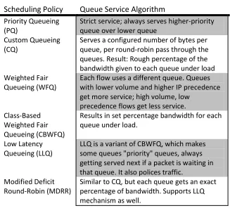
24

the 80th percentile of the individual exponential components, with µ=5.0 and 1.0. The plots are given as a function of the number of components n, which was varied from 1 to 30.

Figure 2.3 Erlang-n versus sum of n exponentials

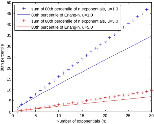
Similar results are given in Figure 2.4 and Figure 2.5, but for the 95th and 99th percentile respectively. The value of µ was set to 1.

0 5 10 15 20 25 30 0

5 10 15 20 25 30 35 40 45 50

Number of exponentials (n)

8

0

th

p

e

rc

e

n

ti

le

sum of 80th percentile of n exponentials, u=1.0 80th percentile of Erlang-n, u=1.0

(41)

25

Finally Figure 2.6, is similar to Figure 2.5, but the number of components was raised from 1 to 100. This was done to see if there are any hidden data patterns as the number of

0 5 10 15 20 25 30 0 10 20 30 40 50 60 70 80 90

Number of exponentials (n), u=1.0

9 5 th p e rc e n ti le

sum of 95th percentile of n exponentials 95th percentile of Erlang-n

0 5 10 15 20 25 30 0 20 40 60 80 100 120 140

(42)

26

components increases. However, the difference between sum and percentile of Erlang-n is still found to be exponentially increasing.

In general, for a given value of µ, the arithmetic sum of the individual cth percentiles is always greater than the cth percentile of the end-to-end distribution, and thus the difference increases as n increases. Also the difference increases as c increases. Finally for a given value of c, the growth of difference between the arithmetic sum of the individual cth percentiles and the cth percentile of the end-to-end distribution for each n is independent of the value of the parameter µ. This observation is substantiated below.

Let xexp be the cexp th percentile of an exponential distribution with rate µ i.e., of a component, and let xErl be the cErl th percentile of an Erlang distribution with n stages, each with parameter µ, i.e., of the end-to-end delay. Then, we have that

(1)

and

0 10 20 30 40 50 60 70 80 90 100

0 50 100 150 200 250 300 350 400 450 500

(43)

27

(2)

Given the values of cexp, cErl and xexp,we are interested in finding out a weight function w such that:

(3)

Equation 1 can be re-written as:

Hence equation 3 becomes:

Putting the value of xErl in equation 2, hence equation 2 becomes:

or

(4)

(44)

28

It should be noted here that cexp need not be the same as cErl, i.e., equation 4 calculates a weight for converting exponential percentile to any Erlang percentile (and vice versa). Also µ is not present in equation 4, confirming our previous observation that the difference between the arithmetic sum of individual cth percentiles and the cth percentile of the end-to-end distribution for each n is independ-to-endent of the value of the parameter µ.

Thus given a fixed parameter µ, equation 3 and 4 give us an exact formula to calculate any percentile of an Erlang distribution (cErl), given a specific percentile of the corresponding exponential distribution (cexp). Figure 2.7 and Figure 2.8 give results for the 95th and 99th percentile respectively. In each figure we plotted x computed using equation 3 and 4 and also using the CDF of the Erlang-n, for n =1,2.3,..,30. As expected, the results are identical.

Figure 2.7 95th percentile of Erlang-n and using weight function

0 5 10 15 20 25 30 0 5 10 15 20 25 30 35 40

(45)

29

Figure 2.8 99th percentile of Erlang-n and using weight function

2.3.2 Exponential Components with different rate parameter

In the case where the rate parameters of the components are not necessarily the same, the end-to-end distribution is a hypoexponential distribution. This can be seen as a generalized Erlang distribution where each stage i has a different rate µi. In general, if we

have n independently distributed exponential random variables Xi, then the random variable,

is hypoexponentially distributed. The hypoexponential has a minimum squared coefficient of variation of 1 / n, and its Laplace transform is:

We note that the PDF and CDF formulas of the hypoexponential distribution are not readily available in the literature. These can be obtained by inverting its Laplace transform as follows. Using partial fraction expansion, we have that:

0 5 10 15 20 25 30 0 5 10 15 20 25 30 35 40 45

(46)

30

We observe that is the Laplace transform of an exponential distribution with parameter µi.

Hence we have,

or

(5)

From equation 5 we can obtain the CDF of a hypoexponential distribution. We have

(6)

The observations made above for the Erlang distribution are also valid for the hypoexponential distribution. In Figure 2.9 we plotted the sum of the 95th percentile of n exponential components, where parameter value of each component is , µi =i, i=1,2,3,…,n

(47)

31

Figure 2.9 Hypoexponential-n versus sum of n exponentials

Figure 2.10 Hypoexponential-n versus sum of n exponentials

It should be mentioned here that the shape of the cth percentile of the hypoexponential distribution depends on the value of the µ parameters. The graphs of Figure 2.9 and Figure 2.10 flatten out as µ gets smaller for each additional component.

The results of equation 3 and 4 can be easily generalized for the hypoexponential case. First consider a hypoexponential with two stages with parameters µ1and µ2. Let xH be

1 2 3 4 5 6 7 8 9 10 2 3 4 5 6 7 8 9

Number of exponentials (n), ui=i,i=1..n

sum of 95th percentile of n exponentials 95th percentile of hypoexponential-n

1 2 3 4 5 6 7 8 9 10 4 5 6 7 8 9 10 11 12 13 14

Number of exponentials (n), ui=i,i=1..n

(48)

32

the cHth percentile of hypoexponential distribution and let xi be the cith percentile of the ith

stage, i=1,2. The CDF is given by:

(7)

Now we can find out the weight function, w, such that:

(8)

Again the CDF of each of the exponential component i can be written as:

or

(9)

Putting the value of xHfrom equation 8 and µi from equation 9 in equation 7, we get

(10)

Given xi and , i=1,2, we can calculate the weight function, w, using the above

expression for any percentile point cH of the two stage hypoexponential. This weight, when

multiplied by the sum of xi, , i=1,2, gives the point xH.

The above expression can easily be generalized as:

(49)

33 and

(12)

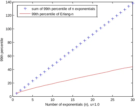
For illustration purposes we plot xH., i.e., the cH.th percentile of the hypoexponential

distribution, calculated using its CDF formula and using the relations given by equation 10 and 11.We have set c =0.95. The plots are identical for any given value ofcH. In Figure 2.11,

the parameters µ1and µ2increase monotonically for each successive observation. In Figure

2.12, parameter µ1 increases and µ2.decreases over the same range hence giving a bowl

shaped output. Both plots coincide.

Figure 2.11 95th percentile of hypoexponential-2 and equation 12

1,2 2,3 3,4 4,5 5,6 6,7 7,8 8,9 9,10 10,11 0 0.5 1 1.5 2 2.5 3 3.5 4

Parameter values: u1,u2

9 5 th P e rc e n ti le o f H y p o e x p o n e n ti a l-2

(50)

34

The results hold for any number of hypoexponential stages. For illustration purposes, we have set n=6 and c =0.95, and the parameters have been varied as follows. In Figure 2.13 . In Figure 2.14, and in Figure 2.15, , for i =1,...,4, parameters µ5 increases and µ6.decreases over the same range for each

successive observation.

1,190 3,17 5,15 7,13 9,11 11,9 13,7 15,5 17,3 19,1

0.5 1 1.5 2 2.5 3 3.5

Parameter values: u1,u2

95th percentile of hypoexp-2 95th percedntile using equation 12

1 2 3 4 5 6 7 8 9 10 0.5 1 1.5 2 2.5 3 3.5 4 4.5 5

Parameter values: u1 (ui=i*u1,i=1,...,6)

(51)

35

2.3.3 Two-stage Coxian

The same idea can be applied to a more generalized distribution, like a two-stage Coxian distribution. We first present a brief review the Phase Type (PH) distribution.

10 11 12 13 14 15 16 17 18 19

25 30 35 40 45 50 55

Parameter values: u1 (ui=i/u1, i=1,...,6)

95th percentile of hypoexp-6 95th percentile using equation 12

5,23 7,21 9,19 11,17 13,15 15,13 17,11 19,9 21,7 23,5

4.5 4.52 4.54 4.56 4.58 4.6 4.62 4.64

Parameter values: u5,u6 (u1=1,u2-2,u3=3,u4=4)

(52)

36

Consider a continuous-time Markov process with n+1 states, where n ≥ 1, such that the states 1,...,n are transient states and state n+1 is an absorbing state. Further, the process has an initial probability of starting in any of the n+1 phases given by the probability vector (α, αn+1), where α is a 1xn vector. Thus the PH distribution is any continuous distribution, X, on [0,∞) which can be obtained as a distribution of time until the absorption state is reached in a continuous time finite state Markov Chain. This process can be written in the form of a generator matrix as follows,

Where S is a 2nx2n transition rate matrix and is defined as: . 0 is a 1xn vector with each element 0 and 1 is an nx1 vector with each element 1. The pair is called a representation function of PH distribution.

The PDF and CDF of a PH distribution are as follows:

Here represents matrix exponential, which is defined as:

(53)

37

Where and are zeroes of the denominator of the rational polynomial. The distribution with the above Laplace transform can be expressed in terms of exponential stages as shown in Figure 2.16

Figure 2.16 Coxian-n distribution

One of the most commonly used Coxian distributions is the two-stage Coxian (C2)

consisting of two phases as shown in Figure 2.17

Figure 2.17 Coxian-2 distribution

The Laplace transform of C2 is given by:

(54)

38

Hence C2 is a special type of PH distribution as this Markov process can be

represented using the rate matrix:

Now let us consider a series of n C2 components connected in tandem as shown in

Figure 2.18

Figure 2.18 A series of Coxian 2 distributions

The end-to-end service time distribution, where each component is a C2, can be

represented by a PH distribution with the following 2nx2n rate matrix:

,

and starting vector , of length n, the PDF and CDF of this PH distribution are:

(55)

39

where 1 is a column vector of size n containing all 1’s and

The CDF of the PH can be solved to get the value of x corresponding to a percentile c using an analytical tool such as Matlab or Mathematica.

Let xe2e be the cth percentile of the PH distribution corresponding to the n component

C2 distribution. Let xi be the cth percentile of the ith C2 stage, i=1,...,n. We are looking for a

weight function w such that:

w (x1 + x2 + … + xn) = xe2e

Following the same steps as before, if the triplet (µ1, µ2, a) is known for

each component, one can calculate the weight function from the expression:

₍₁₃₎

(14)

Here we assume we know the parameters of the individual C2 components. The

(56)

40

Figure 2.19 95th percentile of phase type and equation 14

Figure 2.20 95th percentile of phase type and equation 14

2.4 Inter-provider Quality of Service

A set of recommendations to simplify deployment of inter provider Quality of Service (QoS) for services spanning multiple networks were presented in a white paper [36]. It is

1 2 3 4 5 6 7 8 9 10

0 5 10 15 20 25

Number of C2 components (n), each with u1=1, u2=2, a=b=0.5

P e rc e n ti le o f e n d t o e n d d is tr ib u ti o n

99th percentile of phase type 99th percentile using eq 14 95th percentile of phase type 95th percentile using eq 14 80th percentile of phase type 80th percentile using eq 14 10th percentile of phase type 10th percentile using eq 14

1 2 3 4 5 6 7 8 9 10

0 1 2 3 4 5 6 7

Number of C2 components (n), each with u1=1*n, u2=2*n, a=b=0.5

P e rc e n ti le o f e n d t o e n d d is tr ib u ti o n

(57)

41

well known that providers currently deploy widely differentiated services based on a QoS architecture, such as DiffServ and MPLS. However, enabling QoS based peering among various providers is an area of open research and debate. The document recommends standards and best practices that can help simplify the deployment of QoS for traffic that traverses the network of various providers.

The authors considered three network performance metrics: one way latency (IPTD), one way packet loss (IPLR) and one way delay variation (IPDV) also known as jitter. Also they defined two QoS classes, a single low latency service class and a to best effort class. The low latency class is suitable for applications like VOIP and is consistent with the service class definition of Y.1541 [37]. The parameters specified in Y.1541 are as follows. IPTD is defined as the mean one way end-to-end delay with values ranging from 100 to 400 ms (depending on geographic distance). IPDV or jitter is defined as a percentile of the inter-arrival time of packets at the destinations with 50 ms being the 99th percentile, and the end-to-end packet loss is 1 x 10-3. To support time sensitive traffic with desired QoS in a multi-provider network, the end-to-end performance metrics must be met as specified above.