ABSTRACT
WEI, RAN. Bayesian Variable Selection Using Continuous Shrinkage Priors for Nonparametric Models and Non-Gaussian Data. (Under the direction of Subhashis Ghoshal and Brian Reich.)
In this thesis, we study the properties and applications of Bayesian variable selection in regression models. We focus on Bayesian shrinkage priors that are global-local mixture priors to select an appropriate subset of covariates. First, a Bayesian non-parametric re-gression model is proposed with multivariate continuous shrinkage prior. This approach is to decompose the commonly-used linear regression model into the summation of nonlin-ear main effects and two-way interaction terms and apply the proposed computationally-advantageous continuous shrinkage prior to identify important effects. We construct a multivariate Dirichlet-Laplace prior that aggressively shrinks many of the terms towards zero, thus mitigating the noise of including unimportant exposures and allowing us to isolate the effects of important exposures. Theoretical studies demonstrate the asymp-totic prediction and variable selection consistency properties, while numerical simulations present model performance of prediction and variable selection under practical scenar-ios. The method is applied on neurobehavioral data from Agricultural Health Study that investigates the associations between pesticide use and neurobehavioral outcomes in farmers. The proposed method shows improved accuracy in predicting the joint effects on neurobehavioral responses, while restricting the number of covariates included in the model through variable selection technique.
coefficient estimates are asymptotically concentrated around the true sparse vector in L2-error contraction rate. It is shown that the proposed contraction rate is comparable
with point mass prior that is studied in Atchad´e (2017). The simulation study under logistic regression model verifies the theoretical results by showing that shrinkage priors such as horseshoe prior and Dirichlet-Laplace prior perform quite similar as the point mass prior in estimation, variable selection and prediction, but yield much better results than Bayesian lasso and non-informative normal prior.
©Copyright 2017 by Ran Wei
Bayesian Variable Selection Using Continuous Shrinkage Priors for Nonparametric Models and Non-Gaussian Data
by Ran Wei
A dissertation submitted to the Graduate Faculty of North Carolina State University
in partial fulfillment of the requirements for the Degree of
Doctor of Philosophy
Statistics
Raleigh, North Carolina 2017
APPROVED BY:
Jane Hoppin Soumendra Lahiri
Subhashis Ghoshal
Co-chair of Advisory Committee
Brian Reich
DEDICATION
To my family, To all of my friends,
BIOGRAPHY
ACKNOWLEDGEMENTS
I would like to thank all the people who contributed in some ways during the completion of my thesis and my Ph.D. degree.
First I want to express my appreciation to my co-advisors Dr. Subhashis Ghoshal and Dr. Brian Reich. It has been a pleasure to work with both of them. Dr. Ghoshal is always an excellent example as a responsible and humble scholar. I really appreciate all his dedication of time, ideas and mentoring to make my pursuit of Ph.D. degree always productive and insightful. I am also grateful for the opportunity working with Dr. Reich on the applications and development of statistics methods. Dr. Reich is always fun to work with. His humor, passion and admiration towards academic research have inspired me in different perspectives throughout my entire Ph.D. experience. I would like to express my deepest and most genuine gratitude to their mentorship.
I am also thankful for having Dr. Jane Hoppin and Dr. Soumendra Lahiri as my committee members. I met Dr. Jane Hoppin in an interdisciplinary research project. She showed me a wonderful example of a successful and passionate woman scientist. She has contributed tremendous work in my research project and provided her thoughtful advice outside of the statistical discipline. I would also like to extend my appreciation to Dr. Lahiri for his support and helpful comments on my research projects. He has always been very generous spending his time during the entire process.
comments on my work. The experience of working with them has inspired me to apply my technique skills in statistics to solve real world problems in public health.
I would like to acknowledge the Department of Statistics at North Carolina State University. I am grateful for every faculty member and staff in the department. Their services and dedication have made the department a big family for all the students. My graduate experience benefitted greatly from every course I took, the opportunities of academic research and industrial training, the resources of cutting-edge research in Statistics and the fundings we received to help us continuing our graduate study without financial burden.
TABLE OF CONTENTS
LIST OF TABLES . . . viii
LIST OF FIGURES . . . x
Chapter 1 INTRODUCTION . . . 1
1.1 Bayesian Shrinkage Prior . . . 1
1.2 Notations . . . 3
1.3 Outline of Thesis . . . 4
Chapter 2 Bayesian Shrinkage for Additive Nonparametric Regression 6 2.1 Introduction . . . 6
2.2 Model Description and Prior Specification . . . 9
2.2.1 Main-effect-only model . . . 9
2.2.2 Main and interaction effects model . . . 11
2.2.3 Identifiability constraints . . . 12
2.3 Posterior Sampling . . . 14
2.4 Asymptotic Properties . . . 15
2.4.1 Notations and assumptions . . . 15
2.4.2 Main results . . . 17
2.4.3 Proof of Theorem 2.4.1 and Theorem 2.4.2 . . . 18
2.5 Simulation Study . . . 31
2.5.1 Simulation description . . . 31
2.5.2 Simulation results: main-effect-only model . . . 35
2.5.3 Model with main and interaction effects . . . 36
2.6 Analysis of the AHS Neurobehavioral Dataset . . . 38
2.6.1 Description of the neurobehavioral data . . . 38
2.6.2 Multivariate extension . . . 39
2.6.3 Neurobehavioral data analysis . . . 42
2.7 Conclusion . . . 45
Chapter 3 Contraction Properties of Shrinkage Priors in Logistic Re-gression Model . . . 47
3.1 Introduction . . . 47
3.2 Contraction Results in Logistic Regression . . . 50
3.2.1 Main results . . . 50
3.2.2 Proof of Theorem 3.2.1 . . . 53
3.3 Examples of Shrinkage Priors . . . 62
3.3.1 Spike-and-slab prior . . . 62
3.3.3 Horseshoe prior . . . 66
3.4 Simulation Study . . . 67
3.5 Conclusion . . . 71
Chapter 4 Spatial Shrinkage Prior for Forecasting Calibration . . . 73
4.1 Introduction . . . 73
4.2 Data Description . . . 77
4.2.1 Monitor and forecast data . . . 77
4.2.2 Constructing forecast covariates . . . 78
4.3 Model Description and Prior Specification . . . 79
4.3.1 Spatially-varying nonparametric additive model . . . 79
4.3.2 Gaussian process prior with continuous shrinkage . . . 80
4.3.3 Spatio temporal residual dependence . . . 81
4.4 Posterior Sampling . . . 82
4.5 Simulation Study . . . 84
4.5.1 Simulation design . . . 84
4.5.2 Methods for comparison . . . 86
4.5.3 Simulation results . . . 88
4.6 Implementation to Wildland Fire Smoke Forecasting . . . 90
4.6.1 Computational details . . . 91
4.6.2 Model comparisons . . . 91
4.6.3 Summarizing the calibration results . . . 93
4.7 Conclusion . . . 98
LIST OF TABLES
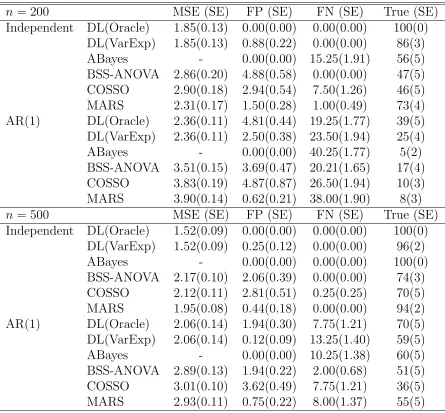
Table 2.1 Summary of the main-effect-only simulation study. Methods are com-pared in terms of mean squared errors (“MSE”), False Positive (“FP”), False Negative (“FN”) and True model (“True”) with their standard er-rors (“SE”) under independent and autoregressive covariate covariance in parentheses. All values except the MSE’s are given in percentages (%). 34 Table 2.2 Summary of simulation study with main and interaction effects.
Meth-ods are compared in terms of mean squared errors (“MSE”), False Pos-itive (“FP”), False Negative (“FN”) and correct selection of main ef-fects, interactions, as well as complete model with their standard errors (“SE”) in parentheses. All values except the MSE’s are given in per-centages (%). . . 38 Table 3.1 Summary of the simulation study that compares the Bayesian logistic
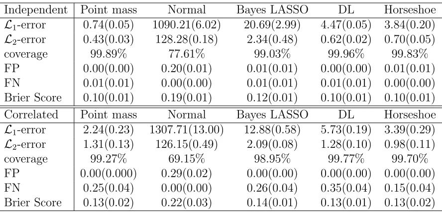
regression models with point-mass prior, non-informative normal prior (Normal), Bayesian LASSO, Dirichlet-Laplace prior (DL) and horse-shoe prior for independent and correlated covariates. The values in parentheses are standard errors. . . 70 Table 4.1 Summary of the simulation study with independent residuals. The
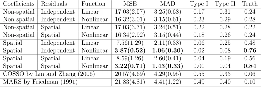
meth-ods vary by whether the additive functions are linear or nonlinear, whether the coefficients β(s) change spatially or not, and whether the errors εt(s) are independent or spatially-correlated. All methods are compared in terms of prediction mean squared error (MSE), prediction mean absolute deviation (MAD), Type I and Type II errors for selec-tion important covariates, and the proporselec-tion of data sets for which true model is selected (Truth). The standard errors are in the parentheses. 89 Table 4.2 Summary of the simulation study with spatially-correlated residuals.
LIST OF FIGURES
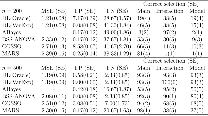
Figure 2.1 (a) Box-plot of the posterior distribution of L2-norm kβj/σk for a single simulated data set; (b) Variation-explained plot at different model sizes for a single data sets (the horizontal red line is the full model “variation - explained” measurement). Note that only the first 20 model sizes are shown in the Figure. . . 33 Figure 2.2 Box-plot for the L2-norm of mean curve basis coefficients kµj/σk. . . 42 Figure 2.3 Average (over Central Nervous System tests) exposure-response curves
¯
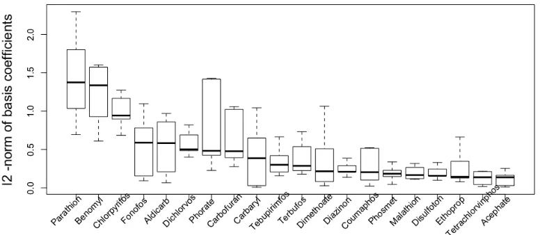
fj(X) for each pesticide in the Agricultural Health Study. The x-axis is the cumulative number of pesticide applications. The solid lines are the posterior means and the dashed lines are point-wise 95% credible intervals. The plots in red are the pesticide covariates selected by DL model. . . 43 Figure 2.4 Posterior distribution of normal variance ωj for average coefficients
across CNS responses. . . 44 Figure 4.1 Monitor station measurements (circles) and forecasts from wildland
fire smoke prediction system (background color) for log 1+PM2.5(µg/m3)
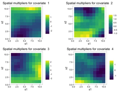
at 2015-08-17 3:00:00GMT (Greenwich Mean Time). The circles in gray are missing monitor measurements. . . 78 Figure 4.2 One example of the spatially-varying multipliers δj(s) for non-zero
covariates in the simulation study. . . 85 Figure 4.3 Box plots of the posteriors of λj (left) and φj (right) j = 1, . . . , p, in
multivariate nonparametric regression model. “Forecast” is the fore-cast at the closest grid point to the monitoring station, covariates with “Mean(r)” are the differences of weighted averages in rings with cur-rent range parameter rkm and previous range parameter (r−10)km, covariates with “Max(r)” are the weighted maximum in the rings with difference range parameters. . . 93 Figure 4.4 Posterior means (red) and 95% credible intervals (grey) of the main
effect curvesfj(X,s), for significant predictors (X1: closest point
fore-cast; X2: difference of weighted average for r1 = 10km and closest
point forecasts; X10: difference of weighted averages for r5 = 50km
and r4 = 40km) at different locations (latitude and longitude shown
in the title). . . 94 Figure 4.5 The maps of absolute correlations between calibrated forecasts under
Figure 4.6 Top: Forecasted values from fire smoke prediction system at 2015-08-17 03:00:00GMT and at 2015-09-15 07:00:00GMT; middle: PM2.5 measurements from monitoring stations; bottom: Calibrated forecasts using nonparametric spatial-temporal model with smooth covariate matrix. All the values are in the scale of log 1 + PM2.5(µg/m3)
Chapter 1
INTRODUCTION
1.1
Bayesian Shrinkage Prior
For statistical models such as linear regression, logistic regression or normal mean mod-els, high-dimensional data analysis is challenging due to its computational burden and the inherent limitations due to the high complexity of the model. Despite the difficulty of high-dimensional data, approximate solutions can be achieved with the assumption of sparsity that restricts the number of important covariates to be small. A variety of regularization methods such as LASSO (Tibshirani, 1996), SCAD (Fan and Li, 2001) and adaptive LASSO (Zou, 2006) have been proposed to identify sparse solutions for high-dimensional analysis.
generally carried out by Reversible Jump Markov Chain Monte Carlo methods (Green, 1995). A spike-and-slab prior (Ishwaran and Rao, 2005) is a mixture of two normal dis-tributions with one highly concentrated at around zero. The Stochastic Search Variable Selection (SSVS) method (George and McCulloch, 1993) can be used to compute the pos-terior distribution corresponding to a spike-and-slab prior. Due to high computational costs, these methods are not scalable to very high dimensional situations commonly aris-ing in recent applications. For high-dimensional model with sparsity assumption, the Bayesian LASSO (Park and Casella, 2008) uses a double exponential prior distribution on the coefficients. The posterior mode of the Bayesian LASSO is the LASSO estima-tor in linear regression model, and the posterior can be computed by a simple Gibbs sampling procedure. However, the Bayesian LASSO does not make the posterior distri-bution concentrate near the true value in large samples (Castillo et al., 2015), although its mode (the LASSO estimator) has good estimation and variable selection properties under appropriate conditions.
point mass prior, the shrinkage priors can be represented as a global-local scale mixtures of Gaussian distribution:
βj ∼N(0, ψjτ), ψj ∼f, τ ∼g, (1.1)
where τ controls the overall shrinkage towards the origin while ψj allows individual deviations for different levels of shrinkage, for j = 1, . . . , p. The dominated peak at zero aggressively shrinks covariates towards zero and the heavy tails avoid over-shrinkage for true signals. These priors are referred to as continuous shrinkage priors, one-component priors or global-local priors. Recent contributions in the literature show their promising posterior concentration properties near the true value and ability to identify true non-zero coefficients. Theoretically, shrinkage priors are shown to obtain almost the same contraction rate as the point-mass prior for recovering the model parameters and the true subset of covariates in the model, for both low-dimensional (Armagan et al. 2013b) and high-dimensional (Song and Liang, 2017) data. It may be noted that under such priors, the posterior probability of hitting the exact value zero is always zero, so some appropriate thresholding procedure needs to accompany the Bayesian procedure.
1.2
Notations
Throughout the thesis, we let β denote the coefficients in our proposed models. Then
β∗ and σ∗2 are the model parameters under the truth. We also let ξ∗ ⊂ {1, . . . , p} be
the indices of covariates with nonzero effects, for example, β∗j 6= 0 for all j ∈ξ∗. In the
theorems and prood, P∗ and E∗ stand respectively for the probability and expectation on
E∗ are represented as Pf∗,σ∗ and Ef∗,σ∗, where f∗ is the true regression mean function.
For the prior density πα(·) with hyper-parameter α, we let Pα(·) be the probability on the model parameters.
For two positive sequences aandb, the relation a≺bmeans lima/b = 0,a&bmeans a/bis bounded below, andab stands form1 <lim infa/b ≤lim supa/b < m2 for some
positive constants m1 and m2.
1.3
Outline of Thesis
In Chapter 2, an additive nonparametric regression model is proposed to investigate the associations between health endpoint and mixture of pesticide exposures. Motivated by neurobehavioral data from Agricultural Health Studies (AHS), we propose a robust regression model to delineate the joint effects of multiple exposures of pesticide. The regression mean function is decomposed as main effects and interaction effects in non-parametric functions, where model uncertainty of each individual function is addressed though B-spline basis expansion and shrinkage priors on the basis coefficients. Specifi-cally, we expand the notion of the computationally efficient Dirichlet-Laplace (DL) prior introduced in Bhattacharya et al. (2015) to multidimensional variation for simultane-ous shrinkage on the basis coefficient vector. We further evaluate the prediction consis-tency and variable selection consisconsis-tency for the proposed nonparametric regression model based on the contraction results in linear regression model with shrinkage priors (Song and Liang, 2017). Furthermore, we incorporate the neurobehavioral data to explore the health effects of multiple pesticide measurements and how the effects on each health endpoint differ from the effects on overall neurobehavioral system.
We consider the incorporation of Bayesian shrinkage prior in logistic regression and com-pare the performance with point-mass prior for recovering the true model parameters. Chapter 3 studies logistic regression model in high-dimensional data. If the shrinkage prior is heavy-tailed and allocates large probability mass in a very small neighborhood of zero, we show that the Bayesian shrinkage prior in logistic regression model achieves optimal contraction rate that can be almost the same as the point-mass prior. The the-oretical results illustrate the advantages of shrinkage priors for their promising posterior consistency and computational efficiency. Examples of shrinkage priors are demonstrated and posterior consistency results can be achieved with certain prior restrictions. The sim-ulation study under logistic regression model verifies the theoretical results by showing that shrinkage priors such as horseshoe prior and Dirichlet-Laplace prior perform quite similar as the point mass prior in estimation, variable selection and prediction.
Chapter 2
Bayesian Shrinkage for Additive
Nonparametric Regression
2.1
Introduction
significance of linear coefficient for each pesticide measurements.
Since the pesticide exposures may have complex nonlinear associations with health endpoints, nonparametric models are preferable considering their robustness to model as-sumptions. Previous literature has introduced different nonparametric regression models to delineate the associations between covariates and response variables and overcome the limitations of linear regression. Friedman (1991) developed multivariate regression splines (MARS) that defines multivariate nonparametric regression model using splines. Lin and Zhang (2006) proposed the component selection and smoothing operator (COSSO) tech-nique that uses penalized regression to select variables. In the Bayesian framework, Lin-kletter et al. (2006) and Savitsky et al. (2011) modeled the response surface as a Gaussian process and used Bayesian variable selection techniques in selecting subset of covariates. Bobb et al. (2014) implemented Bayesian kernel machine regression model that assumes nonparametric associations between mixtures and health response.
as in Curtis et al. (2014) but use a different Bayesian variable selection method.
In this chapter, an additive nonparametric regression model is assumed for both main effect of each pesticide and interaction effect between pesticide mixtures. We deliver two major findings to the existing empirical literature on the health effects of multiple chem-ical exposures. First, we address the uncertainty about the subset of covariates to be included through B-spline basis expansion with multivariate shrinkage prior so that the level of shrinkage on basis coefficients is reported to identify the significant main effects and interactions. Second, we expand the notion of the computationally-efficient Dirichlet-Laplace (DL) prior introduced in Bhattacharya et al. (2015) to multidimensional vectors to achieve simultaneous shrinkage on the basis coefficient vector for each main effect or interaction effect function. Theoretically, we expand the current prediction consistency and variable selection consistency results for shrinkage prior under linear regression model to the proposed additive nonparametric model, where induced bias from B-spline approx-imation and shrinkage on multidimensional vectors pose the major challenges. Further, we incorporate neurobehavioral data from AHS to explore the health effects of multiple pesticides measurements and how the effects on each health endpoint differ from the effects on overall neurobehavioral system.
2.2
Model Description and Prior Specification
2.2.1
Main-effect-only model
We first demonstrate the main-effect-only model that assumes the regression mean func-tion is the summafunc-tion of main effect funcfunc-tions for individual covariate. Let the data be (Y, X), where Y is the response variable denoting the health endpoint, Xn×p = (X1, . . . , Xp)T is a p-vector of chemical exposure measurements. For the nonparamet-ric regression model of Y on the covariatesX, we assume that
Y =µ+f(X1, . . . , Xp) +ε, (2.1)
whereµ is the intercept and the error termε ∼N(0, σ2). Assuming the covariates in the data affect the response variable in mutually independent nonparametric functions, the joint effect is decomposed as the sum of individual main effect functions:f(X1, . . . , Xp) =
Pp
j=1fj(Xj), where fj(Xj) is the univariate nonparametric function of Xj.
If each main effect function of individual covariate is sufficiently smooth, it can be approximated using B-spline basis expansions with a predetermined number of basis functions, m. For the covariate matrix X with elements all scaled to (0,1) interval, each main effect function is approximated by fj(Xj) ≈
Pm
r=1Br(Xj)βjr, where Br(Xj), r = 1, . . . , m, are B-spline basis terms for Xj. With this approximation, the nonlinear effects ofXj is transformed into a linear combination of its basis terms with them-vector basis coefficients βj = (βj1, . . . , βjm)T. The regression model in (2.1) can be written as
Y =µ+ p
X
j=1
m
X
r=1
With the regression model defined in (2.2), model uncertainty and main effect of each covariate Xj are addressed through the basis coefficients βj. The m-vector coefficients
βj’s are assgined multivaraite nromal priors with mean zero and different variance factor-sacross j = 1, . . . , p: βj ind∼ Nm(0, σ2λjIm). The local variance factorsλj’s determine the shrinkage on the m-vector basis coefficients so that the problem of selecting important main effects reduces to shrinkage of the λj’s. Using the Dirichelt-Laplace (DL) prior in Bhattacharya et al. (2015), λj follows an exponential distribution with scale parameter τ φj, whereτ is the global factor that determines the tail of the marginal distribution of λj’s and φj > 0, with Ppj=1φj = 1, is the proportion of variance allocated to covariate Xj. Further, a Dirichlet distribution on φ = (φ1, . . . , φp)T and a gamma distribution on τ are assumed. The hyper-parameter α in Dirichlet distribution controls the level of shrinkage so that smaller α gives more concentration around zero and thus a sparser model. Thus, the uncertainty on each nonparametric main effect function is addressed by the implementation of multivariate DL prior on the B-spline basis coefficients. The Bayesian model on the model parameters is formulated as follows,
βj|λj, σ2 ind
∼ Nm(0, σ2λjIm), j = 1, . . . , p, (2.3) λj|φj, τ
ind
∼ Exp(φjτ), j = 1, . . . , p, (2.4)
φ= (φ1, . . . , φp)T ∼Dirichlet(α, . . . , α), τ ∼Gamma(pα,2). (2.5)
After integrating outλj, we get the marginal prior distribution ofβj givenφj, τ is double exponential distribution denoted as DE(pφjτ /2). In linear regression model, however, the DL prior on coefficient is βj|φj, τ ∼ DE(φjτ). Therefore, for this case, the original DL prior plays more mass at zero than the proposed multivariate extension with only one basis term.
2.2.2
Main and interaction effects model
Assuming the effects of covariates on response are not additive but with two-way inter-actions, the underlying joint function includes both main effects and interinter-actions,
Y =µ+ p
X
j=1
fj(Xj) + p−1 X
k=1
p
X
l=k+1
fkl(Xk, Xl) +ε, (2.6)
where the second-order term fkl(Xk, Xl) represents the interaction effects on health end-point between covariatesXkand Xl. We consider only two-way interactions in this model since higher order interactions are less interpretable and including them will make the computational complexity beyond manageable limits.
Using the B-spline basis expansion described in Chapter 2.2.1 to represent each indi-vidual main effect function, we can use the outer product of the B-spline basis terms for interaction effect functions:
fkl(Xk, Xl)≈ m∗
X
s=1
m∗
X
t=1
Bs∗(Xk)Bt∗(Xl)βklst. (2.7)
Normal priors are placed on the coefficients βklst ind
∼ N(0, σ2λkl), for s, t = 1, . . . , m∗. The DL prior is imposed on the local variance factors λkl:
βkl|λkl, σ2 ind
∼ Nm∗×m∗(0, σ2λklIm∗×m∗), l > k, k = 1, . . . , p−1, (2.8)
λkl|φ∗kl, τ
∗ ind
∼ Exp(φ∗klτ∗), l > k, k = 1, . . . , p−1, (2.9)
φ∗ = (φ12, . . . , φ1p, . . . , φp−1,p)T ∼Dirichlet(α, . . . , α), (2.10) τ∗ ∼Gamma
p(p−1) 2 α,2
, (2.11)
where we assume the same sparsity level α for both main effects and interactions.
2.2.3
Identifiability constraints
The additive model in (2.6) is not uniquely identified without constraints on the func-tionsfj andfkl. For example, adding a constant tofj and subtracting the same constant from fj0 for j 6= j0 gives the same mean regression function but different individual
main effect functions. While other restrictions are possible, we restrict the main effect functions to integrate to zero, R01fj(xj)dxj = 0, j = 1, . . . , p. For the functions of in-teractions, we assume that the bivariate functions integrate to zero in both directions,
R1
0 fkl(xk, xl)dxk = 0 for allxl and R1
0 fkl(xk, xl)dxl= 0 for all xk, so that the main effect
functions are not in the span of the interaction functions. The restrictions on main effect functions can be written as
Z 1
0
fj(x)dx=
Z 1
0 " m
X
r=1
βjrBr(x)
#
dx= m
X
r=1
βjr
Z 1
0
Br(x)dx
def
= m
X
r=1
βjrDr = 0, (2.12)
where Dr
def
= R1
restriction on the basis coefficient βj,Pm
r=1βjrDr= 0. For the B-spline basis,
Dr =
r/[d(m−d+ 1)], r= 1, . . . ,(d−1), 1/(m−d+ 1), r=d, . . . ,(m−d+ 1), (m−r+ 1)/[d(m−d+ 1)], r= (m−d+ 2), . . . , m,
where m is the number of B-spline basis functions and d is the degree of B-spline basis. The restrictions on each bivariate function of interactions are also treated as linear constraints on the coefficients for the B-spline expansion in (2.7):
Z 1
0
fkl(xk, xl)dxk = m∗ X s=1 m∗ X t=1 Z 1 0
Bs∗(xk)dxk
Bt∗(xl)βklst
def
= m∗
X
t=1
Bt∗(xl)
m∗ X
s=1
Ds∗βklst
= 0,
(2.13)
Z 1
0
fkl(xk, xl)dxl = m∗ X s=1 m∗ X t=1
Bs∗(xk)
Z 1
0
Bt∗(xl)dxl
βklst def = m∗ X s=1
Bs∗(xk)
m∗ X
t=1
D∗tβklst
= 0,
(2.14)
where we assume Ds∗ def= R1 0 B
∗
s(x)dx for s = 1, . . . , m
∗. The restrictions in (2.13) and
(2.14) hold for all xk and xl if an only if
m∗ X
s=1
D∗sβklst =0, for all t= 1, . . . , m∗; m∗
X
t=1
D∗tβklst =0, for all s= 1, . . . , m∗.
2.3
Posterior Sampling
We now describe the computational algorithm for the main-effect-only model. The regres-sion model with both main and interaction effects in the mean function is very similar. We sample the parameters using the combination of Gibbs sampling and direct sampling. The sampler cycles through (i) β|λ, φ, τ, Y, X, (ii)λ|β, φ, τ, Y, X and (iii) φ, τ|λ,β, Y, X. Within step (iii), it follows direct sampling of (iiia) τ|φ, λand (iiib)φ|λ.
(i) Given λj,Y and Xj, the conditional posterior distribution forβj ism-dimensional multivariate normal with mean µβ
j and variance matrix Σβj, where
µβj =
B(Xj)TB(Xj) + Im λj
−1
B(Xj)T Y − p
X
l=1,l6=j
B(Xl)βl
!
, (2.15)
Σβj =
B(Xj)TB(Xj) + Im λj
−1
σ2. (2.16)
For the restrictions on basis coefficients in (2.12), we sample βj Pm
r=1βjrDr = 0 from
conditional multivariate normal Nm(µ∗βj,Σ ∗
βj), where
µ∗βj =µβj −ΣβjD(D
TΣ βjD)
−1DTµ
βj, (2.17)
Σ∗β
j =Σβj −ΣβjD(D
TΣ βjD)
−1DTΣ
βj, (2.18)
where D= (D1, . . . , Dm)T.
(ii) Givenφj, τ andβj, the variance componentλj is sampled from generalized inverse Gaussian distribution GiG1− m
2, 2
φjτ,
βTjβj
σ2
.
(iiia) Givenφ1, . . . , φp and λ1, . . . , λp , the global parameter τ in DL prior is sampled from generalized inverse Gaussian distribution GiGp(α−1), 1, 2Pp
j=1
λj
φj
.
general-ized inverse Gaussian distribution GiG(α−1, 1, 2λj) and then let φj =Tj/Ppl=1Tl.
2.4
Asymptotic Properties
In this section, we will study the asymptotic properties of the additive nonparametric regression model for individual main effects with the multivariate DL prior. Since pre-dictors are considered deterministic in our setting, extension to include interactions is similar except that the model will be more complicated. For asymptotic properties, we denote pand m aspn and mn respectively to reflect that they are increasing in n.
2.4.1
Notations and assumptions
For a fixedn×pn covariate matrixX = (X, . . . , Xpn), we consider the additive
nonpara-metric model Y = Ppn
j=1fj(Xj) +σε, where each additive function is approximated by B-spline basis expansion:fj(Xj) =B(Xj)βj+σδ, whereB(Xj) = (B1(Xj), . . . , Bmn(Xj))
is the n×mn matrix of basis terms for Xj and δ denotes the bias induced from basis expansion approximation. Therefore, the true additive regression model is represented as
Y = pn X
j=1
B(Xj)βj +σδ+σε
def
= B(X)β+σδ +σε,
whereB(X) = [B(X1), . . . , B(Xpn)] is the n×pnmn matrix for B-spline basis expansion
terms, β = (βT1, . . . ,βTp n)
T is the p
nmn-vector with each mn-dimensional components corresponding to each covariate Xj and ε is an n-dimensional standard normal vector. We study a Bayesian approach based on a continuous shrinkage prior that selects the nonzero vectors among the mn-dimensional vectors β1, . . . ,βpn. After integrating out
j = 1, . . . , pn,
βj|λj, σ2 ind
∼ Nm(0, λjσ2Im), (2.19)
λj|ψj ind
∼ Exp(ψj), ψj ∼Gamma(α,2). (2.20)
We assume the density function on βj is denoted asπα(βj) with hyper-parameterα. We letf∗j(·) be the true function for covariateXj,β∗ andσ∗be the true values of parameters,
ξ∗ ⊂ {1, . . . , pn} be the indices of covariates with nonzero effects such that f∗j(Xj) 6= 0 for j ∈ξ∗, and the true sparsity level iss∗ =|ξ∗|.
Next we state some regularity conditions on the eigen structure of the B-spline basis expansion matrix B(X) with respect to the sequence {n}, which will be defined later. These assumptions are similar as those in Song and Liang (2017) where they presented the asymptotic properties of shrinkage priors in the linear regression model. The difference lies in the fact that we are dealing with the design matrix of basis terms, and each additive nonparametric function is estimated by B-spline basis expansion so that estimation bias is introduced.
• A1(1): The data dimensionality satisfies that mnpn≥n
• A1(2): Assume κ is the minimum smoothness parameter for all additive functions,
so that the bias induced by mn-dimensional basis expansion is δ m−nκ
• A1(3): The rank of B(X) isn and B(X)TB(X) hasn positive eigenvalues denoted
asnd1/mn, . . . , ndn/mn, whered1, . . . , dn are bounded away from zero
• A1(4): There exists some integer ¯p and a fixed constant d00 with ¯pmnlogpn n2n, such that for any q ≤ p, the basis expansion sub-matrix ˜¯ B(X) consisting qmn columns ofB(X), dmin
˜
• A2(1): {n} sequence is assumed to satisfy that s∗mnlogpn ≺n2n and nm−nκ
• A2(2): minj∈ξ∗ nkβ
∗j/σ∗k √
mn o
n and maxj
nkβ ∗j/σ∗k √
mn o
≤ γ3E for fixed γ3 ∈ (0,1),
and E is nondecreasing with n
• A3: There exists an integer ¯p, which depends on n and pn, and two constants d and d00 such that ¯pmnlogpn n2n and nd0/mn ≥ dmax
˜
B(X)TB˜(X) ≥ dmin
˜
B(X)TB˜(X) ≥ nd00/mn for any q ≤ p¯ and any sub-matrix ˜B(X) of the basis expansion matrix B(X)
Note that assumptionA1(3) is an extension of linear regression model in Song and Liang
(2017), by replacing covariate matrix X to B-spline basis design matrix B(X). From LemmaA.9 in Yoo and Ghosal (2016), we combine the B-spline property with the linear regression model assumption, soA1(3) is specified. The assumption in A2(1) restrictsn to be max(ps∗mnlogpn/n, m−nκ).
2.4.2
Main results
For the nonparametric function defined in the regression model where no model parameter is assumed, we want to demonstrate that the consistency holds for the prediction on the joint effects of covariates. Therefore, the following theorem proves that, when the B-spline basis expansion is implemented, the prediction performance of B(X)β is asymptoticly concentrated around the additive mean function under the truth.
Theorem 2.4.1 For the regression modelY =Pmn
j=1fj(Xj)+σε=B(X)β+σδ+σε, the
basis expansion bias satisfies that kδk √nm−κ
n , where κ is the smoothness parameter.
Assume the assumptions in A1, A2 and A3 hold for the design matrix B(X) and the
((2.20)) with αp−n(1+ν) for ν >0, then we conclude the posterior concentration of the
predictive distribution,
P∗ Pα
B(X)β−
pn X
j=1
f∗j(Xj)
≥c0
√ nn
X, Y
≥e−c1n2n !
≤e−c2n2n, (2.21)
for some constants c0, c1 and c2.
Theorem 2.4.1 shows posterior concentration rate √nn for the predictions at the ob-servation points. Therefore, for the covariates matrix X, the predictionB(X)β obtained from the regression model has concentration rate close to√nmax{ps∗mnlogpn/n, m−nκ} in probabilities around the true mean functionPpn
j=1f∗j(Xj).
Theorem 2.4.2 Denote the subset model by ξ(an) = {j : kβj/σk > an} for nanpn ≺ logpn. Assume the conditions in Theorem 2.4.1 hold and minj∈ξ∗kβ∗jk/
√
mnn, then
P∗
Pα(ξ(an) = ξ∗|X, Y)>1−p−µ 00
n
>1−p−nµ0, (2.22)
for some positive constants µ0 and µ00.
Theorem 2.4.2 shows the posterior variable selection consistency given that an ≺ logpn/npn and the prior density is moderately flat at nonzero basis coefficients β∗j/σ∗.
2.4.3
Proof of Theorem 2.4.1 and Theorem 2.4.2
the multivariate Dirichlet-Laplace (DL) prior, we want to show that it concentrates within a small neighborhood around zero with a dominated and steep peak, while retaining heavy tails away from zero.
Lemma 2.4.3 For any positive constant µ >0 and thresholding value an ≤
q
d0
0
mnn/pn,
1−
Z
kβ|≤an
πα(β)dβ≤p−n(1+µ), (2.23)
if the Dirichlet parameter satisfies αp−n(1+ν) for ν > µ.
Proof For a vector β of dimensionmn, the prior density is defined in (2.19) and (2.20). When λ is given, T def= kβk2/λ∼χ2
mn. Next, we have
1−
Z
kβk≤an
πα(β)dβ=
Z ∞ 0 Z ∞ 0 P
T > a
2
n λ
p(λ|ψ)pα(ψ)dψdλ
=
Z a2n/pn 0
P
T > a
2
n λ
Z ∞
0
p(λ|ψ)pα(ψ)dψ
dλ
+
Z ∞
a2
n/pn
P
T > a
2
n λ
Z ∞
0
p(λ|ψ)pα(ψ)dψ
dλ (2.24)
For any constantµ > 0, we can conclude that
Z a2n/pn 0
P
T > a
2
n λ
Z ∞
0
p(λ|ψ)pα(ψ)dψ
dλ≤P(T > pn)Pα(λ < a2n/pn)≤e−pn/2, (2.25) where the last inequality is obtained from the tail property of χ2-distribution.
Next, from Lemma 3.3 in Bhattacharya et al. (2015), it follows that
Z ∞
a2
n/pn
P
T > a
2
n λ
Z ∞
0
p(λ|ψ)pα(ψ)dψ
for a constant C1 >0. Combining the inequalities in (2.24), (2.25) and (2.26), we have
1−
Z
kβk≤an
πα(β)dβ≤e−pn/2+C1αlog(pn/a2n)≤p
−(1+µ)
n .
for αp−n(1+ν) where ν > µ.
Lemma 2.4.4 For a small constant η >0 and E defined in assumption A2(2),
−log
Z
Ppn−s∗ j=1 kβjk≤η
√
mnn
pn−s∗ Y
j=1
πα(βj)dβ1. . . dβpn−s∗ !
≺n2n, (2.27)
−log
inf
kβk≤√mnE
πα(β)
≺n2n/s∗. (2.28)
Proof When λj is given, the mn-dimensional vector βj satisfies that kβjk/
p
λj
iid
∼χmn
for j = 1, . . . , pn. Therefore, for the prior of λj defined in (2.20),
E(kβjk) = E
E kβjkλj
= EpλjE(kβjk/
p
λj
λj)
= √
2Γ((mn+ 1)/2) Γ(mn/2)
E(pλj), (2.29) and then E(pλj) = E
E(pλj|ψj)
= Γ(3/2)E(pψj) = Γ(3/2)
√
2Γ(α+1/2)
Γ(α) . Then for a
constant C2 >0 free of α, E(kβjk) = C2
√
mnα. By the Central Limit Theorem,
Pα
pn−s∗ X
j=1
kβjk √
mn ≤ηn
!
= Pα
1 pn−s∗
pn−s∗ X
j=1
kβjk √
mn
≤ ηn pn−s∗
!
≥1/2 (2.30)
if α≤ C3n
pn−s∗, which can be verified since αp −(1+ν)
n for ν > 0. Therefore, we show that
−log
Z
Ppn−s∗ j=1
kβjk √
mn≤ηn
pn−s∗ Y
j=1
πα(βj)dβ1. . . dβpn−s∗ !
We need to prove that −log infkβk≤√mnEπα(β)
≺n2
n/s∗. For s1/s2 close to zero,
inf
kβk≤√mnE
πα(β) =
Z ∞
0 Z ∞
0
(2πλ)−mn/2e−mnE2/2λp(λ|ψ)p
α(ψ)dλdψ ≥(2πs2)−mn/2e−mnE
2/2s 1P
α(s1 < λ < s2). (2.32)
As λ follows prior distribution in (2.20) for a given hyper-parameter α, we have
Pα(s1 < λ < s2) = Z ∞
0
(e−s1/ψ−e−s2/ψ)p
α(ψ)dψ≥ e−s2/2
Γ(α)(s2−s1)
Z s2
0
ψα−2e−s2/ψdψ ≥αe−s2/2(s
2−s1)s −(1−α) 2
Z ∞
1
t−αe−tdt ≥C4α(1−s1/s2)e−s2/2
for a constant C4 >0. Therefore, whenmn/s1 ≺nn2/s∗ and s2 ≺n2n/s∗, we have
−log
inf
kβk≤√mnE
πα(β)
≤ mn
2 log(2πs2)+ mnE2
2s1
+(1+ν) logpn+s2/2≺n2n/s∗. (2.33)
Lemma 2.4.5 The prior density πα(βj/σ) satisfies
max j∈ξ∗
sup
kx1k,kx2k∈[kβ∗j/σk− √
mnC0n,kβ∗j/σk+ √
mnC0n]
πα(x1) πα(x2)
< ln, (2.34)
for a constant C0 >0 and s∗logln ≺logpn.
Proof By assumption, minj∈ξ∗
kβ√∗j/σ∗k
mn > n, maxj∈ξ∗
kβ√∗j/σ∗k
mn < E and
πα(x) =
Z ∞
0 Z ∞
0
φ(x|λ)p(λ|ψ)pα(ψ)dψdλ =
Z ∞
0
(2πλ)−mn/2e−kxk2/2λ Z ∞
0
where the function of λ in integrand f∗(λ) def= (2πλ)−mn/2e−kxk2/2λ is concave and it is
increasing on (0,kxk2/m
n] and decreasing on (kxk2/mn,∞). Then we can separate the integral by kxk2/m
nlogpn so thatf∗(λ) is increasing until the point kxk2/mn. Since
Z kxk2/mnlogpn 0
f∗(λ)
Z ∞
0
p(λ|ψ)pα(ψ)dψdλ≤
2πkxk2
mnlogpn
−mn/2
e−mnlogpn/2 (2.35) Z ∞
kxk2/m
nlogpn
f∗(λ)
Z ∞
0
p(λ|ψ)pα(ψ)dψdλ≥
Z kxk2/mn 2kxk2/m
nlogpn
f∗(λ)
Z ∞
0
p(λ|ψ)pα(ψ)dψdλ
≥(2πkxk2/m
n)−mn/2e−mnlogpn/2Pα
2k
xk2
mnlogpn
< λ < kxk
2
mn
≤C5(2πkxk2/mn)−mn/2e−mnlogpn/4αe−kxk 2/2m
n. (2.36)
AndC5 >0 is constant free of n. The inquality in (2.36) is obtained from the conlcusion
in the proof of Lemma 2.4.4. Then for mn > n2n, we can prove that
Rkxk2/mnlogpn
0 f
∗(λ)R∞
0 p(λ|ψ)pα(ψ)dψdλ R∞
kxk2/m
nlogpnf
∗(λ)R∞
0 p(λ|ψ)pα(ψ)dψdλ
≤ (logpn)
mn/2e−mnlogpn/2
C5e−mnlogpn/4αe−kxk
2/2m
n
=exp
−logC5+
mn
2 log logpn−
mnlogpn
4 + (1 +ν) logpn+ kxk2
2mn
≤exp
−C50n2n
for a constant C50 > 0. The proved inequality on the ratio implies that, for a given
x such that kxk2/√m
n ∈ (n, E), the prior density of x has the dominated mass on λ∈(kxk2/m
nlogpn,∞):
πα(x)
R∞ kxk2/m
nlogpn R∞
0 φ(x|λ)p(λ|ψ)pα(ψ)dψdλ
1. (2.37)
such that kx1k < kx2k, πα(x1) and πα(x2) have dominated mass on the interval λ ∈
(s3,∞), where s3 def
= min kx1k2/mnlogpn,kx2k2/mnlogpn
. Then we have
ln= max j∈ξ∗
sup
kx1k,kx2k∈kβ∗j/σ∗k±C0
√
mnn
πα(x1)
πα(x2)
max j∈ξ∗
sup
kx1k,kx2k∈kβ∗j/σ∗k±C0
√
mnn R∞
s3
R∞ 0
φλ(x1) φλ(x2)
φλ(x2)p(λ|ψ)pα(ψ)dψdλ
R∞
s3
R∞
0 φλ(x2)p(λ|ψ)pα(ψ)dψdλ
= max j∈ξ∗
sup
kx1k,kx2k∈kβ∗j/σ∗k±C0
√
mnn R∞
s3
R∞ 0 e
1 2λ(kx2k
2−kx 1k2)φ
λ(x2)p(λ|ψ)pα(ψ)dψdλ
R∞
s3
R∞
0 φλ(x2)π(λ|ψ)πα(ψ)dψdλ
≤max j∈ξ∗
sup
kx1k,kx2k∈kβ∗j/σ∗k±Co √
mnn
exp
1 2s3
kx2k2− kx1k2
≤max j∈ξ∗
exp
n
2mn(kβ∗j/σ∗k/
√
mn+C0n)C0n/s3 o
.
Whenkx1k ≥ kx2k, then we haveln≤1, which is obvious to prove thats∗logln≺logpn. Therefore, we only consider the situation when kx1k < kx2k. And we have s∗logln ≤ C6s∗mnEn/s3 for constant C6 > 0. Therefore, given that s∗mnn ≺ logpn, we have s∗logln ≺logpn. Thus prove the Lemma.
The three lemmas above specify the conditions on prior concentration properties. Lemma 2.4.3 and Lemma 2.4.4 establish that the prior probability that the L2-norm
of each basis coefficient larger than an is arbitrarily small with the constraint: an ≤
p
Proof of Theorem 2.4.1 We follow the results of Theorem A.1 and Theorem A.2 in Song and Liang (2017), but the difference is that we have additional bias,
Y = p
X
j=1
fj(Xj) +σε=B(X)β+σδ+σε, (2.38)
where each additive function is estimated bymn-dimensional basis expansion. Therefore, Y includes both bias term and linear regression part analogous to the model in Song and Liang (2017). The linear coefficient β = (β1, . . .βpn)T is a p
n ×mn-dimensional basis coefficient vector where a multivariate DL prior will be imposed for each covariate. The true model is the additive non-parametric model Pp
j=1f∗j(Xj) +σ∗ε, wheref∗j 6= 0 are κ−smooth functions for j ∈ ξ∗ and f∗j = 0 are zero effects for j /∈ ξ∗. In our proposed
model, we estimate each function by basis expansion B(Xj)βj, which imposes an extra bias term δ in (2.38) due to approximation error. The magnitude of δ is bounded by a multiplier ofm−κ
n .
ForBn={At least ˜pof kβj/σkis larger than an}formnp˜n2n/logpnandmnp˜n≺ n2
n, Cn ={kB(X)β−
Pp
j=1f∗j(Xj)k ≥σ∗n} ∪ {σ2/σ2∗ >(1 +n)/(1−n)} ∪ {σ2/σ2∗ <
(1−n)/(1 +n)} and An =Bn∪Cn, we first consider test function φn= max{φ0n,φ˜n},
φ0n = _
{ξ⊃ξ∗,|ξ|≤p˜+s∗}
1
YT(I−H ξ)Y (n−mn|ξ|)σ2∗
−1 ≥c
0 0n
˜ φn =
_
{ξ⊃ξ∗,|ξ|≤p˜+s∗}
1
kB(Xξ) B(Xξ)TB(Xξ)
−1
B(Xξ)TY −
X
j∈ξ
f∗j(Xj)k ≥˜c0σ∗
√ nn/5
for sufficiently large constants c00 and ˜c0, where Hξ = B(Xξ) B(Xξ)TB(Xξ)
−1
B(Xξ)T is the hat matrix corresponding to the subgroup ξ, and P
satisfies ξ⊃ξ∗, mn|ξ| ≤mn(˜p+s∗)≺n2n,
E(f∗,σ∗2)1
YT(I−H ξ)Y (n−mn|ξ|)σ∗2
−1
≥c00n
=E(f∗,σ∗2)1
εT(I−H ξ)ε n−mn|ξ|
−1 + 2ε
T(I −H ξ)δ n−mn|ξ|
+ δ T
(I−Hξ)δ n−mn|ξ|
≥c00n
≤P(f∗,σ∗2)
εT(I−Hξ)ε−(n−mn|ξ|)
+ 2
εT(I−Hξ)δ
+δT(I−Hξ)δ ≥(n−mn|ξ|)c00n
.
Since the magnitude of basis expansion bias is in the order of m−nκ, we have
δT(I −Hξ)δ ≤kδk2 nm−n2κ ≺(n−mn|ξ|)n 2εT(I −Hξ)δ ≤2kδk · kεk 2
√
nm−nκkεk.
For normally distributed error ε, given the property of chi-square distribution, we have
P(f∗,σ∗2) 2
εT(I−Hξ)δ
≥(n−mn|ξ|)c00n
≤P r kεk ≥c000nm2nκ2n ≺exp{−c0000n2n}.
Combining with the conclusion in (A.3) of Song and Liang (2017), we can prove that
E(f∗,σ∗2)1
YT(I −Hξ)Y (n−mn|ξ|)σ∗2
−1
≥c00n
≤exp{−c3n2n}. (2.39)
Next, f∗j(Xj) can be approximated by B-spline basis expansion B(Xj)β∗j with bias term δ, whereβ∗j is the basis coefficients for the true non-parametric function. We have
B(X)β− pn X
j=1
f∗j(Xj)
=B(X)(β−β∗)−δ
≤B(Xξ)(βξ−β∗ξ) +
B(Xξc)βξc +
where B(Xξ)(βξ − β∗ξ)
≤
√
nβξ − β∗ξ,
B(Xξc)βξc
≺
√
nanpn ≺ √
nn and
δ≺
√
nn. By the condition thatmn(˜p+s∗)≺n2n, we have, for some constantc
0 3,
E(f∗,σ∗2)1
kB(Xξ) B(Xξ)TB(Xξ)
−1
B(Xξ)TY −
X
j∈ξ
f∗j(Xj)k ≥c˜0σ∗
√ nn/5
=E(f∗,σ∗2)1
B(Xξ)(βξ−β∗ξ)− X
j∈ξ
f∗j(Xj)−B(Xξ)βξ
≥c˜0σ∗
√ nn/5
≤E(f∗,σ∗2)1
B(Xξ)TB(Xξ)
−1
B(Xξ)TY −βξ
≥˜c00σ∗n/5 ≤E(f∗,σ∗2)1
B(Xξ) B(Xξ)TB(Xξ) −1
B(Xξ)Tε+ B(Xξ)TB(Xξ)
−1
B(Xξ)Tδ
≥˜c0n/5
≤exp(−c03n2n), (2.40)
where the inequality is given by (A.4) of Song and Liang (2017) and the fact that kδk √nm−nκ. Therefore, combining (2.39) and (2.40), we can prove that E(f∗,σ2∗)φn ≤
exp(−˜c3n2n) for some fixed ˜c3, according to (A.5) in Song and Liang (2017).
For the additive model, the process to prove that sup(β,σ2)∈C
nEβ(1−φn) is similar as
the proof of Theorem A.1 in Song and Liang (2017), by replacing their covariate matrix X with B(X). Therefore, we have inequalities
E(f∗,σ2∗)φn≤exp(−cn 2
n) (2.41)
sup
(β,σ2)∈C
n
E(β,σ2)(1−φn)≤exp(−c0n2n). (2.42)
The next step is to show that
lim n Pf∗,σ
2
∗
nm(Dn)
L∗(Dn)
≥exp(−c4n2n)
o
>1−exp{−c5n2n}, (2.43)
out the parameters on their priors and L∗(Dn) is the likelihood under the truth so that
m(Dn) L∗(Dn)
=
Z
(σ∗)nexp{−kY −B(X)βk2/2σ2}
σnexp{−kY −Ppn
j=1f∗j(Xj)k2/σ∗2}
π(β, σ2)dβdσ2.
From the proof of Theorem A.1 in Song and Liang (2017), we only need to show that, conditional on 0≤σ2 −σ2
∗ ≤η02n, for some constants c5 and c6,
Pf∗,σ∗2 Pα
kY −B(X)βk2/2σ2 < Y −
pn X
j=1
f∗j(Xj)
2
σ2∗+c5n2n
≥e−c6n2n !
≥1−exp(−c5n2n).
For our proposed model, each element in B(X) is smaller than 1 and kδk2 nm−2κ n ≺ n2
n. By the property of chi-square distribution and normal distribution, with probability larger than 1−exp{−c5n2n}, we havekεk2 ≤n(1 +c
0
5),kεTB(X)k∞≤c 0
5nnfor constant c05. Then for model parameters (β, σ2), we have
{kY −B(X)βk2/2σ2 <kY −(f∗1(X1) +. . .+f∗pn(Xpn))k 2
/σ∗2+c5n2n} ={kεσ∗/σ+B(X)(β∗−β)/σ+δσ∗/σk2 <kεk2+ 2c5n2n}
⊃{kB(X)(β∗−β)/σk<pkεk2+ 2c
5n2n−(σ∗/σ)kεk −(σ∗/σ)kδk} ⊃n
pn X
j=1
k(β∗j−βj)/σk ≤2η√mnn
o
⊃nkβj/σk ∈
kβ∗j/σk −η√mnn/s∗,kβ∗j/σk+η √
mnn/s∗
for all j ∈ξ∗ o
∩n X j /∈ξ∗
kβj/σk ≤η√mnn
o
.
for some constant η. The second subset relation is given by Assumption A1(3) such that
the eigenvalues ofB(X)TB(X) are in the same order as n/m
2.4.3 and Lemma 2.4.4,
Pα
X
j /∈ξ∗
βj/σ≤η
√ mnn
0≤σ2 −σ∗2 ≤η02n
=
Z
Ppn−s∗ j=1 kβjk≤η
√
mnn
pn−s∗ Y
j=1
π(βj)dβ1. . . dβpn−s∗ ≥exp{−c06n2n}
Pα
kβj/σk ∈
kβ∗j/σk −η√mnn/s∗,kβ∗j/σk+η √
mnn/s∗
|{0≤σ2−σ2∗ ≤η02n}
≥ηn· inf
kβk≤√mnE
πα(β)/s∗ ≥exp{−c006n2n}.
Thus verify the inequality in (2.43).
Finally, from the proof of Theorem A.1 in Song and Liang (2017), forBndefined above, we have Pα(Bn)< e−c7n
2
n for some constants c
7, given that R
kβk>anπα(β)dβ≤p −(1+µ)
n .
Combining the results of Pα(Bn)< e−c7n 2
n with (2.41), (2.42) and (2.43), we have
Pf∗,σ∗2 π
B(X)β−
pn X
j=1
f∗j(Xj)
≥σ∗
√
nn or|σ2−σ∗2|> c4n
X, Y
≥e−c1n2n !
≤e−c2n2n.
In conclusion, the results in Theorem 2.4.1 is proved.
Proof of Theorem 2.4.2 The proof of Theorem 2.4.2 follows the proof of Theorem A.3 in Song and Liang (2017). Note that in our proposed model, we have basis expansion matrix B(X) instead of covariate matrix X, the coefficients vector β = (βT1, . . . ,βTp
n)
T
are shrunk within blocks β1, . . . ,βpn. Furthermore, our model has an additional bias term δ due to B-spline basis expansion.
inf(β,σ2)∈S
1π(β, σ
2)/π(σ2), π(β|σ2) = sup
(β,σ2)∈S
1π(β, σ
2)/π(σ2). The maximum of L 2
-norm for each group within coefficient vector is defined as kβkmax 4
= maxjkβjk. We can conclude by proof of Theorem A.3 in Song and Liang (2017),
Pα(ξ=ξ∗|X, Y)&π
β(ξ∗)c
σ
max≤an
π(βξ∗|σ2)
q
det(B(Xξ∗)TB(Xξ∗))
−1√2πs
× inf
kβ(ξ∗)ckmax≤an(σ∗+c2n)
Γ(a0+ (n−s)/2)
SSE(β(ξ∗)c)/2 +b0
a0+(n−s)/2, (2.44)
where SSE(β(ξ∗)c) is the SSE when β(ξ∗)c is given and fixed.
Next, we let kβkmin 4
= minkβjk be the minimum of L2-norms for each predictor
within coefficient vector. Similarly, we can show that
Pα(ξ=ξ0|X, Y). π
βξ0\ξ ∗ σ min
> an,
β(ξ0)c
σ
max
≤an
π(βξ∗|σ2)qdet(B(X
ξ∗)TB(Xξ∗)) −1
×√2π
s
sup
kβ(ξ0)ckmax≤an(σ∗+c2n)
Γ(a0+ (n−s)/2)
SSE(β(ξ0)c)/2 +b0
a0+(n−s)/2.
where SSE(β(ξ0)c) is the SSE when β(ξ0)c is given and fixed.
Due to the basis expansion biasδsuch thatkδk2 nm−2κ
n , we can the same derivation as (A.13) and (A.14) of Song and Liang (2017). With probability larger than 1−4pn·p
−c06 n ,
SSE(β(ξ∗)c) =(Y −B(X(ξ∗)c)β(ξ ∗)c)
T(I−H
ξ∗)(Y −B(X(ξ∗)c)β(ξ∗)c)
≤σ2∗εT(I−Hξ∗)ε+σ 2
∗δT(I −Hξ∗)δ+
B(X(ξ∗)c)β(ξ∗)c 2
+ 2σ∗2p2c06nlogpn
X
j∈(ξ∗)c
kβjk; (2.45)
SSE(β(ξ0)c)≥σ2∗εT(I−Hξ0)ε+σ∗2δT(I −Hξ0)δ−2σ∗ p
2c06nlogpn
X
j∈(ξ0)c
and with probability 1−p−c
00
6
n for any constantc006, we have
εT(I−Hξ∗)ε−ε
T(I−H
ξ0)ε ≤c0
7mn|ξ0\ξ∗|logpn.
Since δT(I−Hξ∗)δ−δ
T
(I−Hξ0)δ ≤c007mn|ξ0 \ξ∗|nm−n2κ, we can conclude that
supkβ
(ξ∗)ckmax≤an(σ∗+c2n)(SSE(β(ξ∗)c)/2 +b0)
a0+(n−s)/2 infkβ(ξ0)ckmax≤an(σ∗+c2n)(SSE(β(ξ0)c)/2 +b0)a0+(n−s)/2
≤e{c08mn|ξ0\ξ∗|logpn+c008mn|ξ0\ξ∗|nm−n2κ}. (2.47)
If mn (lognpn)1/2κ, we have nm−n2κ ≺ logpn, so that the right hand side of (2.47) is c8mn|ξ0 \ξ∗|logpn. Given (2.34) in Lemma 2.4.5, π(βξ∗|σ
2)/π(β
ξ∗|σ
2) ≤ ls
n. We can proceed with
Pα(ξ=ξ0|X, Y) Pα(ξ=ξ∗|X, Y)
≤lnsσ∗+c2n σ∗−c2n
[pn−(1+µ)/(1−pn−(1+µ))]|ξ0\ξ∗|
e{c8mn|ξ0\ξ∗|logpn} ≤ls
n
σ∗+c2n σ∗−c2n
p−µ0mn|ξ0\ξ∗|
n ,
with proper choice of the constants. Therefore, with minj∈ξ∗kβjk
√
mnn, according to the proof of Theorem A.2 in Song and Liang (2017), we can prove that
X
ξ0 )ξ∗
Pα(ξ =ξ0|X, Y)≤Pα
kβ−β∗k>
minj∈ξ
∗
kβjk −anσ
X, Y
≤e−cn2n
In conclusion, we have Pf∗,σ2
∗ n
Pα ξ(an) =ξ∗|X, Y
>1−p−µ00 n
o
>1−p−µ0
2.5
Simulation Study
In the simulation study, we evaluate model performance in terms of both prediction and variable selection. We first consider the additive nonparametric regression model that only includes individual main effects as in Chapter 2.2.1, and then expand the regression model to include two-way interaction effects as in Chapter 2.2.2.
2.5.1
Simulation description
For the simulated data, the number of covariates isp= 50 and the sample size is fixed at either n= 200 or n = 500. For the covariate matrix X, we first sample Xj∗,j = 1, . . . , p, from Gaussian distribution with E(Xj∗) = 0, Var(Xj∗) = 1 and Cov(Xj∗, Xk∗) = 0 for mutually independent case or Cov(Xj∗, Xk∗) = 0.5|j−k| for autoregressive case. Next, the
simulated random vectors are rescaled onto the unit interval by Xj = X∗
j−min(Xj∗) max(Xj∗)−min(Xj∗).
Given the covariate matrixX, the responseY is generated from normal distribution with mean f(X)def= f1(X1) +f2(X2) +f3(X3) +f4(X4) and variance σ2 = 1.5, where
f1(x) = e1.1x
3
−2 f2(x) = 2x−1,
f3(x) = sin(4πx), f4(x) = log{(e2−1)x+ 1} −1.
The remaining p−4 predictors have no effect on the response.
prediction accuracy is evaluated by mean squared error (MSE) on a testing data:
MSE = 1 500
500 X
i=1
f(x0i1, . . . , x0ip)−fˆ(x0i1, . . . , x0ip)2, (2.48)
where f(·) is the true mean function for covariate matrix, ˆf is the estimated mean function, Xi0 = (x0i1, . . . , x0ip)T are a new data randomly sampled from the proposed covariate distribution,i= 1, . . . ,500. Note thatXi0’s are not used for model fitting but for evaluating the model prediction performance. Therefore, we can compare the prediction performance of each method on future observations.
We also record the variable selection performance for correctly identifying the four significant covariates. We evaluate variable selection results in terms of the percentage of unimportant variables selected (False Positive) and the percentage of important variables excluded (False Negative), averaged over all the simulated data sets under each scenario. We also include the proportion of the simulated data sets in which the true model is selected (Truth). However, for the multivariate DL prior the factors fj(·) will never equal zero exactly. Therefore, a thresholding policy is needed for variable selection. We implement a thresholding technique based on the idea that choosing a subset of predictors so that the corresponding prediction deterioration in terms of “variation-explained” can be tolerated (Hahn and Carvalho, 2015). Given the posterior samples of coefficients βj, the posterior samples of the “variation-explained” values for are calculated as
V(k) =
kPp
j=1B(Xj)βjk2 kPp
j=1B(Xj)βjk2+nσ2 +k
Pp
j=1B(Xj)βj −
Pp
j=1B(Xj)β (k)
j k2
, (2.49)
(a)
(b)
Figure 2.1: (a) Box-plot of the posterior distribution of L2-norm kβj/σk for a single simulated data set; (b) Variation-explained plot at different model sizes for a single data sets (the horizontal red line is the full model “variation - explained” measurement). Note that only the first 20 model sizes are shown in the Figure.
posterior median of V(k) with 80% intervals at different model sizes k = 1, . . . ,20. The
shrinkage level for variable selection will be determined by the smallestk so that the 80% interval of Vk includes the posterior mean of full modelV50 (red line in Figure 1(b)). We
Table 2.1: Summary of the main-effect-only simulation study. Methods are compared in terms of mean squared errors (“MSE”), False Positive (“FP”), False Negative (“FN”) and True model (“True”) with their standard errors (“SE”) under independent and au-toregressive covariate covariance in parentheses. All values except the MSE’s are given in percentages (%).
n
= 200
MSE (SE)
FP (SE)
FN (SE)
True (SE)
Independent
DL(Oracle)
1.85(0.13)
0.00(0.00)
0.00(0.00)
100(0)
DL(VarExp)
1.85(0.13)
0.88(0.22)
0.00(0.00)
86(3)
ABayes
-
0.00(0.00)
15.25(1.91)
56(5)
BSS-ANOVA
2.86(0.20)
4.88(0.58)
0.00(0.00)
47(5)
COSSO
2.90(0.18)
2.94(0.54)
7.50(1.26)
46(5)
MARS
2.31(0.17)
1.50(0.28)
1.00(0.49)
73(4)
AR(1)
DL(Oracle)
2.36(0.11)
4.81(0.44)
19.25(1.77)
39(5)
DL(VarExp)
2.36(0.11)
2.50(0.38)
23.50(1.94)
25(4)
ABayes
-
0.00(0.00)
40.25(1.77)
5(2)
BSS-ANOVA
3.51(0.15)
3.69(0.47)
20.21(1.65)
17(4)
COSSO
3.83(0.19)
4.87(0.87)
26.50(1.94)
10(3)
MARS
3.90(0.14)
0.62(0.21)
38.00(1.90)
8(3)
n
= 500
MSE (SE)
FP (SE)
FN (SE)
True (SE)
Independent
DL(Oracle)
1.52(0.09)
0.00(0.00)
0.00(0.00)
100(0)
DL(VarExp)
1.52(0.09)
0.25(0.12)
0.00(0.00)
96(2)
ABayes
-
0.00(0.00)
0.00(0.00)
100(0)
BSS-ANOVA
2.17(0.10)
2.06(0.39)
0.00(0.00)
74(3)
COSSO
2.12(0.11)
2.81(0.51)
0.25(0.25)
70(5)
MARS
1.95(0.08)
0.44(0.18)
0.00(0.00)
94(2)
AR(1)
DL(Oracle)
2.06(0.14)
1.94(0.30)
7.75(1.21)
70(5)
DL(VarExp)
2.06(0.14)
0.12(0.09)
13.25(1.40)
59(5)
ABayes
-
0.00(0.00)
10.25(1.38)
60(5)
BSS-ANOVA
2.89(0.13)
1.94(0.22)
2.00(0.68)
51(5)
COSSO
3.01(0.10)
3.62(0.49)
7.75(1.21)
36(5)
MARS
2.93(0.11)
0.75(0.22)
8.00(1.37)
55(5)
the value of “variation-explained”.
multi-variate DL prior (DL method) to each data set and compare with four competing methods assuming additive nonparametric functions: approximate Bayesian method (“ABayes”) by Curtis et al. (2014); the Bayesian smoothing splines ANOVA (“BSS-ANOVA”) by Reich et al. (2009); component selection and smoothing operator (“COSSO”) by Lin and Zhang (2006) and multivariate adaptive regression splines model (“MARS”) by Friedman (1991). We also implement the “Oracle” selection in DL method which selects the four covariates with largest posterior medians of kβj/σk. With the correct information on the number of significant covariates, this DL oracle method will demonstrate the ability of the general DL method to rank important covariates and formally select significant ones. For DL model and BSS-ANOVA where MCMC sampling is implemented, the total sampling iteration is 15,000 with 5,000 burn-in steps.
2.5.2
Simulation results: main-effect-only model
(2.49), it might have uncertainty in determining the number of important covariates, but when the number is fixed like in the Oracle method, DL method will correctly rank the covariates so that higher variable selection accuracy will be achieved. For the others, ABayes is too conservative in choosing subset of covariates with false positive equal to zero for every case and thus large false negative proportion. In the dependent case, ABayes has perfect selection for the larger sample size, but the true model proportions drop considerably when the sample size is less. BSS-ANOVA and COSSO have similar variable selection performance. Their performance for independent data is worse than the competitors and the computation time for BSS-ANOVA is more than three times that of the DL prior method. MARS, on the other hand, performs poorly for correlated data as in the AR(1) case. Overall, the DL method outperforms the competitors, especially in more difficult setting with small sample size and correlated exposures.
2.5.3
Model with main and interaction effects
We also conduct simulation for additive models with both main effects and interactions. Since adding interactions will increase the dimensionality significantly, we reduce the number of covariates to p = 10 and only investigate the independent case. Therefore, there are 10 main effects and 45 interaction effects. The response variable Y is simulated from the model
Y =f1(X1) +f2(X3) +f3(X1X3) +ε,
where is a random number generated from standard normal distribution and functions f1, f2 and f3 are the same as in Chapter 2.5.2. As in the simulation for the
main-effect-only model, we assume the sample size is n= 200 or n= 500.
functionfj(Xj) with B-spline basis functions of orderm= 10 and the two-way interaction functions fkl(Xk, Xl) with the outer product of basis terms of order m∗ = 5 for each covariate. We implement the DL method as described in Chapter 2.2.2 and select the important main and interaction effects using the “variation-explained” criterion, similar to the main-effect-only model. The DL method is compared with ABayes, BSS-ANOVA, COSSO and MARS methods on both prediction performance and variable selection. The accuracy of model prediction is evaluated by computing mean squared error (MSE) for a newly generated covariate matrix, while variable selection is determined by False Negative, False Positive and the percentages of correctly identifying the main effects, interactions and the complete model. For MARS, we use the functionpolymars(·) in the R package polspline. In ABayes and COSSO where interactions are not considered in the available code, the interaction terms are represented as the product of two covariates, that is, we define 45 new covariates Xl·Xk and then use the main effects model with 55 additive predictors for both main effects and interaction terms. The simulation results are summarized in Table 2.2.